2.13.8. Other Papers
Miscellaneous short examples from various texts.
2.13.8.1. Contents
2.13.8.2. Wang on the Wang Transform
Source paper: Wang [2000].
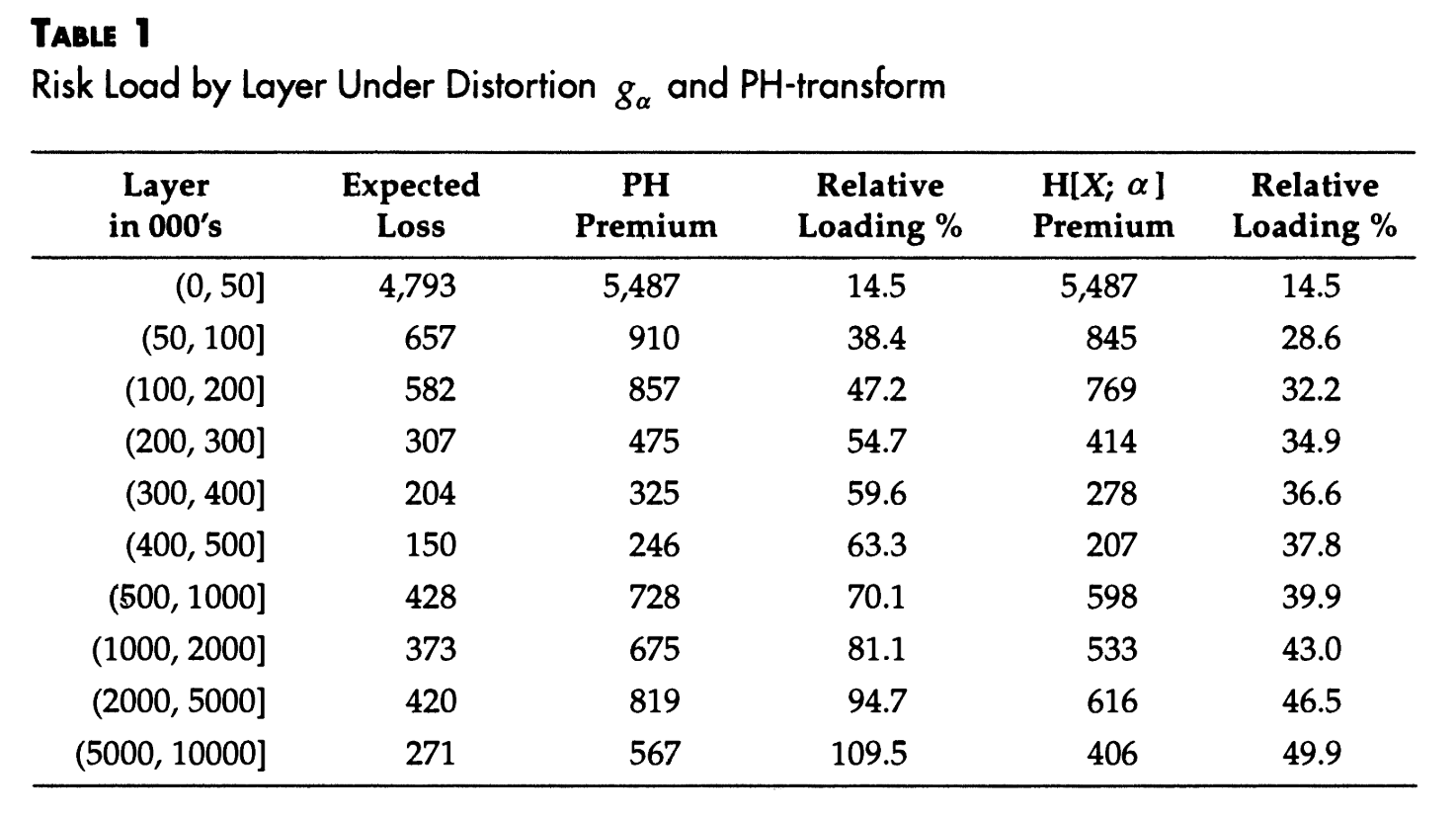
2.13.8.2.1. Pricing by Layer
Concepts: Layer expected loss and risk adjusted layer technical premium with Wang and proportional spectral risk measures.
Setup: Ground-up Pareto risk, shape 1.2, scale 2000. Layer and compare Wang(0.1) and PH(0.9245) pricing.
Source Exhibits:
Thanks: Zach Eisenstein of Aon.
Code:
Build the portfolio.
In [1]: from aggregate import build, qd

In [2]: layers = [0, 50e3, 100e3, 200e3, 300e3, 400e3, 500e3, 1000e3, 2000e3, 5000e3, 10000e3]

In [3]: a1 = build('agg Wang.t1 '
   ...:            '1 claim '
   ...:            '10000e3 xs 0 ' # limit the severity to avoid infinite variance
   ...:            'sev 2000 * pareto 1.2 - 2000 '
   ...:            f'occurrence ceded to tower {layers} '
   ...:            'fixed'
   ...:           )
   ...:

In [4]: qd(a1)

       E[X] Est E[X]    Err E[X]  CV(X) Est CV(X) Skew(X) Est Skew(X)
X
Freq      1                           0
Sev  8179.5   8178.5 -0.00012201 11.595    11.596  70.841      70.841
Agg  8179.5   8178.5 -0.00012201 11.595    11.596  70.841      70.841
log2 = 16, bandwidth = 200, validation: n/a, reinsurance.
Expected loss and other ceded statistics by layer.
In [5]: ff = lambda x: x if type(x)==str else (
   ...:         f'{x/1e6:,.1f}M' if x >= 500000 else
   ...:         (f'{x:,.3f}' if x < 100 else f'{x:,.0f}'))
   ...:

In [6]: fp = lambda x: f'{x:.1%}'

In [7]: qdl = lambda x: qd(x, index=False, line_width=200, formatters={'pct': fp},
   ...:                    float_format=ff, col_space=10)
   ...:

In [8]: qdl(a1.reinsurance_occ_layer_df .xs('ceded', 1, 1).droplevel(0).reset_index(drop=False))

     limit     attach         ex         cv         en   severity        pct
    50,000      0.000      4,787      1.908      1.000      4,787      58.5%
    50,000     50,000        657      8.058      0.020     32,776       8.0%
   100,000    100,000        582     12.148      0.009     65,143       7.1%
   100,000    200,000        307     17.279      0.004     78,055       3.8%
   100,000    300,000        204     21.484      0.002     83,955       2.5%
   100,000    400,000        150     25.182      0.002     87,349       1.8%
      0.5M       0.5M        428     31.751      0.001    324,046       5.2%
      1.0M       1.0M        373     48.091      0.001       0.6M       4.6%
      3.0M       2.0M        420     76.476      0.000       1.7M       5.1%
      5.0M       5.0M        271        126      0.000       3.2M       3.3%
      infM        gup      8,179     11.596      1.000      8,179     100.0%
ZE provided function to make the exhibit table. The column pct shows the relative loading.
In [9]: def make_table(agg, layers):
   ...:     agg_df = agg.density_df
   ...:     layer_df = agg_df.loc[layers, ['F', 'S', 'lev', 'gS', 'exag']]
   ...:     layer_df['layer_el'] = np.diff(layer_df.lev, prepend = 0)
   ...:     layer_df['premium'] = np.diff(layer_df.exag, prepend = 0)
   ...:     layer_df['pct'] = layer_df['premium'] / layer_df['layer_el'] - 1
   ...:     layer_df = layer_df.rename_axis("exhaust").reset_index()
   ...:     layer_df['attach'] = layer_df['exhaust'].shift(1).fillna(0)
   ...:     qdl(layer_df.loc[1:, ['attach', 'exhaust', 'layer_el', 'premium', 'pct']])
   ...:
Make the distortions and apply. First, Wang.
In [10]: d1 = build('distortion wang_d1 wang 0.1')

In [11]: a1.apply_distortion(d1)

In [12]: make_table(a1, layers)

    attach    exhaust   layer_el    premium        pct
     0.000     50,000      4,787      5,481      14.5%
    50,000    100,000        657        845      28.6%
   100,000    200,000        582        769      32.2%
   200,000    300,000        307        414      34.9%
   300,000    400,000        204        278      36.6%
   400,000       0.5M        150        207      37.8%
      0.5M       1.0M        428        598      39.9%
      1.0M       2.0M        373        533      43.0%
      2.0M       5.0M        420        616      46.5%
      5.0M      10.0M        271        406      49.9%
Make the distortions and apply. Second, PH.
In [13]: d2 = build('distortion wang_d2 ph 0.9245')

In [14]: a1.apply_distortion(d2)

In [15]: make_table(a1, layers)

    attach    exhaust   layer_el    premium        pct
     0.000     50,000      4,787      5,480      14.5%
    50,000    100,000        657        910      38.4%
   100,000    200,000        582        856      47.2%
   200,000    300,000        307        475      54.7%
   300,000    400,000        204        325      59.6%
   400,000       0.5M        150        246      63.3%
      0.5M       1.0M        428        727      70.1%
      1.0M       2.0M        373        675      81.1%
      2.0M       5.0M        420        818      94.7%
      5.0M      10.0M        271        567     109.5%
It appears the layer 50000 xs 0 is reported incorrectly in the paper.
2.13.8.2.2. Satellite Pricing
Concepts: The cost of a Bernoulli risk with a 5% probability of a total loss of $100m using Wang(0.1) distortion.
Thanks: Zach Eisenstein of Aon.
Code:
Build the portfolio. Illustrates how to set up a Bernoulli.
In [16]: a2 = build('agg wang2 0.05 claims dsev [100] bernoulli')

In [17]: qd(a2)

      E[X] Est E[X]   Err E[X]  CV(X) Est CV(X) Skew(X) Est Skew(X)
X
Freq  0.05                     4.3589            4.1295
Sev    100      100          0      0         0
Agg      5        5 8.8818e-16 4.3589    4.3589  4.1295      4.1295
log2 = 8, bandwidth = 1, validation: not unreasonable.
Check the distribution output.
In [18]: qd(a2.density_df.query('p_total > 0')[['p_total', 'F', 'S']])

       p_total    F    S
loss
0.0       0.95 0.95 0.05
100.0     0.05    1    0
Build and apply the distortion. Use the price() method. The first argument selects the 100% quantile for pricing, i.e., the limit is fully collateralized. First with the Wang from above. The relative loading reported is the complement of the loss ratio.
In [19]: qd(a2.price(1, d1))

statistic  L      P      M      Q   a      LR       PQ     ROE
line
wang2      5 6.1191 1.1191 93.881 100 0.81712 0.065179 0.01192
Try with a more severe distortion.
In [20]: d3 = build('distortion wang_d2 wang 0.15')

In [21]: qd(a2.price(1, d2))

statistic  L     P     M      Q   a      LR       PQ      ROE
line
wang2      5 6.269 1.269 93.731 100 0.79758 0.066883 0.013539
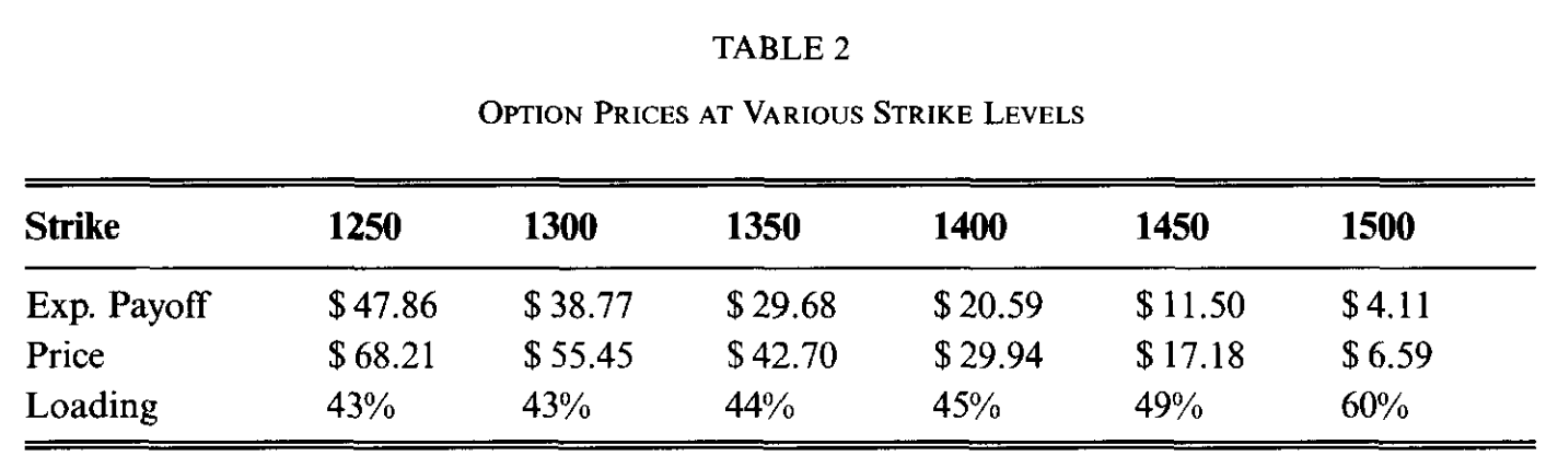
2.13.8.3. Wang on Weather Derivatives
Source paper: Wang [2002].
Concepts: Applying Wang transform to empirical distribution via an Aggregate object.
Source Exhibits:
Data:
Create a dataframe from the heating degree days (HDD) history laid out in Table 1.
In [22]: d = '''Dec-79
   ....: 972.5
   ....: Dec-87
   ....: 1018.5
   ....: Dec-95
   ....: 1199.5
   ....: Dec-80
   ....: 1147.0
   ....: Dec-88
   ....: 1155.0
   ....: Dec-96
   ....: 1156.0
   ....: Dec-81
   ....: 1244.0
   ....: Dec-89
   ....: 1474.5
   ....: Dec-97
   ....: 1040.0
   ....: Dec-82
   ....: 901.0
   ....: Dec-90
   ....: 1129.5
   ....: Dec-98
   ....: 940.5
   ....: Dec-83
   ....: 1573.0
   ....: Dec-91
   ....: 1077.5
   ....: Dec-99
   ....: 1090.5
   ....: Dec-84
   ....: 1055.0
   ....: Dec-92
   ....: 1129.5
   ....: Dec-00
   ....: 1517.5
   ....: Dec-85
   ....: 1488.0
   ....: Dec-93
   ....: 1090.5
   ....: Dec-86
   ....: 1065.5
   ....: Dec-94
   ....: 938.5'''
   ....:

In [23]: import pandas as pd

In [24]: d = d.split('\n')

In [25]: df = pd.DataFrame(zip(d[::2], d[1::2]), columns=['month', 'hdd'])

In [26]: df['hdd'] = df.hdd.astype(float)

In [27]: qd(df.head())

    month    hdd
0  Dec-79  972.5
1  Dec-87 1018.5
2  Dec-95 1199.5
3  Dec-80   1147
4  Dec-88   1155

In [28]: qd(df.describe())

         hdd
count     22
mean  1154.7
std   193.37
min      901
25%   1043.8
50%     1110
75%   1188.6
max     1573
Code:
Create an empirical aggregate based on the HDD data.
In [29]: hdd = build(f'agg HDD 1 claim dsev {df.hdd.values} fixed'
   ....:             , bs=1/32, log2=16)
   ....:

In [30]: qd(hdd)

       E[X] Est E[X]   Err E[X]   CV(X) Est CV(X) Skew(X) Est Skew(X)
X
Freq      1                           0
Sev  1154.7   1154.7 2.2204e-16 0.16362   0.16362 0.95984     0.95984
Agg  1154.7   1154.7 2.2204e-16 0.16362   0.16362 0.95984     0.95984
log2 = 16, bandwidth = 1/32, validation: not unreasonable.
Build the distortion and apply to call options at different strikes. Reproduces Table 2.
In [31]: from aggregate.extensions import Formatter

In [32]: d1 = build('distortion w25 wang .25')

In [33]: ans = []

In [34]: strikes = np.arange(1250, 1501, 50)

In [35]: bit = hdd.density_df.query('p_total > 0')[['p_total']]

In [36]: for strike in strikes:
   ....:     ser = bit.groupby(by= lambda x: np.maximum(0, x - strike)).p_total.sum()
   ....:     ans.append(d1.price(ser, kind='both'))
   ....:

In [37]: df = pd.DataFrame(ans, index=strikes,
   ....:                  columns=['bid', 'el', 'ask'])
   ....:

In [38]: df.index.name = 'strike'

In [39]: df['loading'] = (df.ask - df.el) / df.el

In [40]: qd(df.T, float_format=Formatter(dp=2, w=8))

strike      1250     1300     1350     1400     1450     1500
bid        32.01    25.84    19.67    13.51     7.34     2.44
el         47.86    38.77    29.68    20.59    11.50     4.11
ask        68.21    55.45    42.70    29.94    17.18     6.59
loading    42.5%    43.0%    43.8%    45.4%    49.4%    60.1%
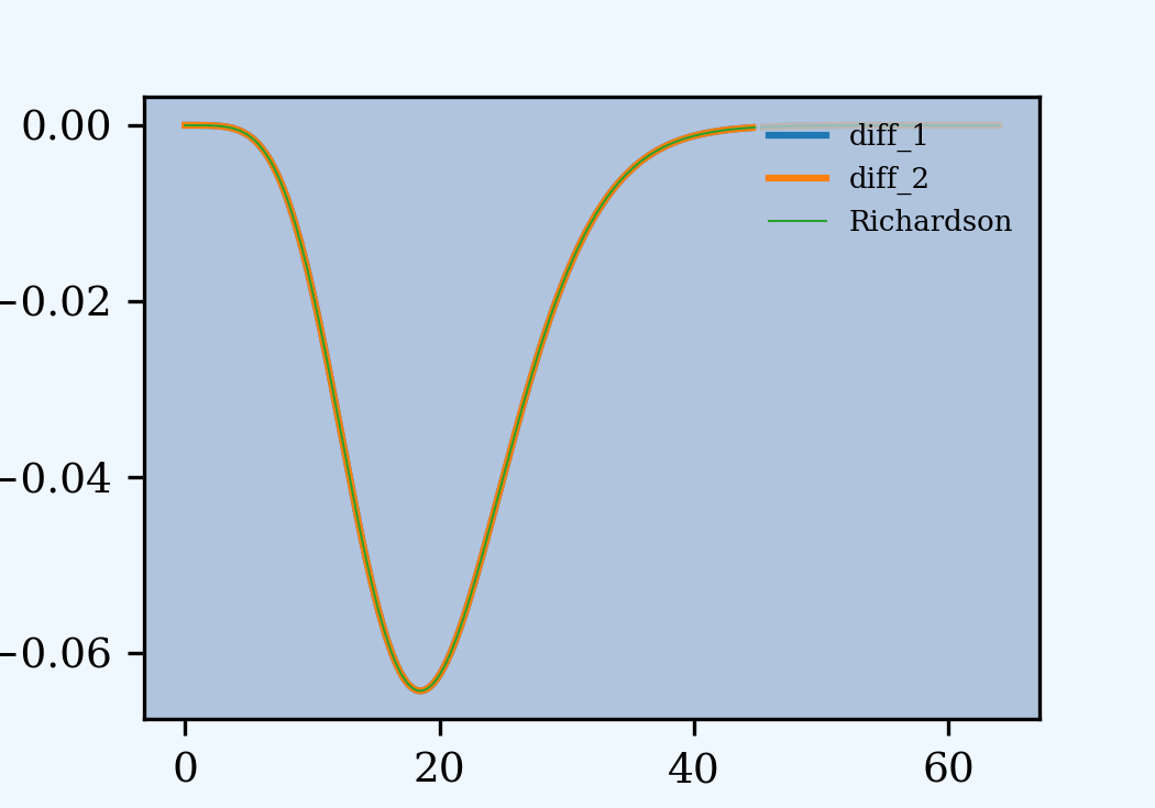
2.13.8.5. Richardson’s Deferred Approach to the Limit
Source papers: Embrechts et al. [1993], Grübel and Hermesmeier [2000].
Concepts: Given estimators of an unknown quantity \(A^* = A(h) + ch^\alpha + O(h^\beta)\) with \(\alpha < \beta\). Evaluate at \(h\) and \(h/t\). Multiply the estimate at \(h/t\) by \(t^\alpha\), subtract the original estimate, and rearrange to get
The truncation error order of magnitude has decreased. The constant \(c\) need not be known. Applying this approach to estimate the density as pmf divided by bucket size, \(f_{h} / h\), Embrechts et al. [1993] report the following.
Setup: Poisson(20) exponential aggregate.
Source Exhibits: Figure 1.
The variable egp3 is treated as the exact answer. It could also be approximated using the series expansion, but this has been shown already, in REF. Set up basic portfolios evaluated at different bucket sizes.
In [56]: egp1 = build('agg EGP 20 claims sev expon 1 poisson',
   ....:             bs=1/16, log2=10)
   ....:

In [57]: qd(egp1)

      E[X] Est E[X]    Err E[X]   CV(X) Est CV(X)  Skew(X) Est Skew(X)
X
Freq    20                      0.22361            0.22361
Sev      1  0.99984 -0.00016274       1    1.0005        2       1.998
Agg     20   19.997 -0.00016277 0.31623    0.3163  0.47434     0.47429
log2 = 10, bandwidth = 1/16, validation: fails sev mean, agg mean.

In [58]: egp2 = build('agg EGP 20 claims sev expon 1 poisson',
   ....:             bs=1/32, log2=11)
   ....:

In [59]: qd(egp2)

      E[X] Est E[X]    Err E[X]   CV(X) Est CV(X)  Skew(X) Est Skew(X)
X
Freq    20                      0.22361            0.22361
Sev      1  0.99996 -4.0689e-05       1    1.0001        2      1.9995
Agg     20   19.999 -4.0713e-05 0.31623   0.31625  0.47434     0.47432
log2 = 11, bandwidth = 1/32, validation: not unreasonable.

In [60]: egp3 = build('agg EGP 20 claims sev expon 1 poisson',
   ....:              log2=16)
   ....:

In [61]: qd(egp3)

      E[X] Est E[X]    Err E[X]   CV(X) Est CV(X)  Skew(X) Est Skew(X)
X
Freq    20                      0.22361            0.22361
Sev      1        1 -1.5895e-07       1         1        2           2
Agg     20       20 -1.5895e-07 0.31623   0.31623  0.47434     0.47434
log2 = 16, bandwidth = 1/512, validation: not unreasonable.
Concatenate and estimated densities from pmf. Compute errors to egp3. Compute the Richardson extrapolation. It is indistinguishable from egp3. The last table shows cases with the largest errors.
In [62]: import pandas as pd

In [63]: df = pd.concat((egp1.density_df.p_total, egp2.density_df.p_total, egp3.density_df.p_total),
   ....:           axis=1, join='inner', keys=[1, 2, 3])
   ....:

In [64]: df[1] = df[1] * 16;                   \
   ....: df[2] = df[2] * 32;                   \
   ....: df[3] = df[3] * (1<<10);              \
   ....: df['rich'] = (4 * df[2] - df[1]) / 3; \
   ....: df['diff_1'] = df[1] - df[3];         \
   ....: df['diff_2'] = df[2] - df[3];         \
   ....: m = df.diff_2.max() * .9;             \
   ....: ax = df[['diff_1', 'diff_2']].plot(figsize=(3.5, 2.45));      \
   ....: (df['rich'] - df[3]).plot(ax=ax, lw=.5, label='Richardson');
   ....:

In [65]: ax.legend(loc='upper right')
Out[65]: <matplotlib.legend.Legend at 0x71a3d41d7fa0>

In [66]: qd(df.query(f'diff_2 > {m}').iloc[::10])

Empty DataFrame
Columns: [1, 2, 3, rich, diff_1, diff_2]
Index: []