2.6. Reinsurance Pricing
Objectives: Applications of the Aggregate class to reinsurance exposure rating, including swings and slides, aggregate stop loss and swing rated programs, illustrated using problems from CAS Parts 8 and 9.
Audience: Reinsurance pricing, broker, or ceded re actuary.
Prerequisites: DecL, underwriting and reinsurance terminology, aggregate distributions, risk measures.
See also: The Reinsurance Clauses, Individual Risk Pricing. For other related examples see Published Problems and Examples, especially Bahnemann Monograph.
Contents:
2.6.1. Helpful References
2.6.2. Basic Examples
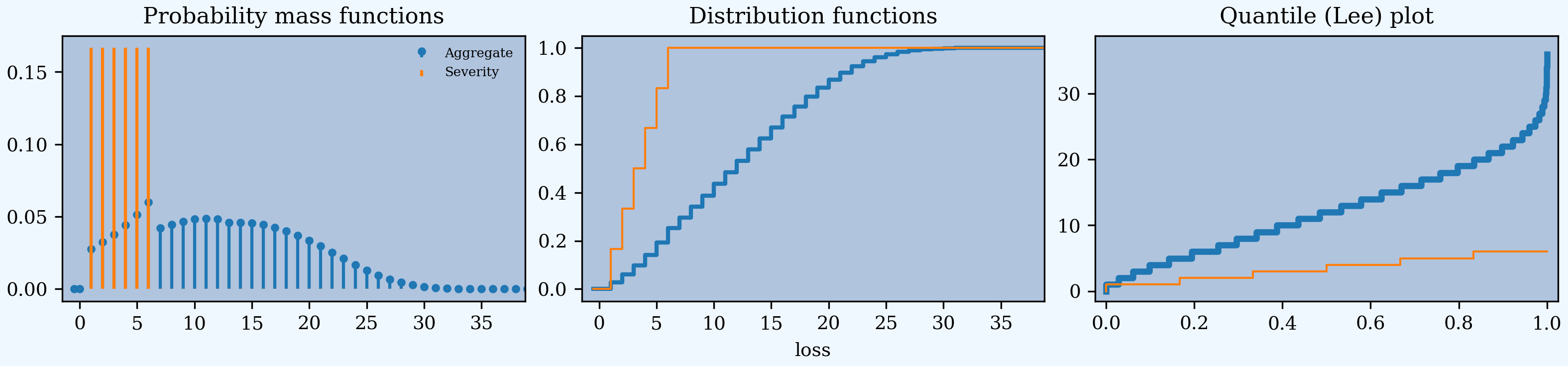
Here are some basic examples. They are not realistic, but it is easy to see what is going on. The subsequent sections add realism. The basic example gross loss is a “die roll of dice rolls”: roll a die, then roll that many dice and sum, see Student. The outcome is between 1 (probability 1/36) and 36 (probability 1/6**7), as confirmed by this output.
In [1]: import pandas as pd

In [2]: from aggregate import build, qd

In [3]: a01 = build('agg Re:01 '
   ...:             'dfreq [1 2 3 4 5 6] '
   ...:             'dsev [1 2 3 4 5 6] ')
   ...:

In [4]: a01.plot()

In [5]: qd(a01)

      E[X] Est E[X]   Err E[X]   CV(X) Est CV(X)  Skew(X) Est Skew(X)
X
Freq   3.5                     0.48795                  0
Sev    3.5      3.5          0 0.48795   0.48795        0  2.8529e-15
Agg  12.25    12.25 1.5543e-15 0.55328   0.55328  0.28689     0.28689
log2 = 7, bandwidth = 1, validation: not unreasonable.

In [6]: print(f'Pr D = 1:  {a01.pmf(1) : 11.6g} = {a01.pmf(1) * 36:.0f} / 36\n'
   ...:       f'Pr D = 36: {a01.pmf(36):8.6g} = {a01.pmf(36) * 6**7:.0f} / 6**7')
   ...:
Pr D = 1:    0.0277778 = 1 / 36
Pr D = 36: 3.57225e-06 = 1 / 6**7
An occurrence excess of loss reinsurance layer is specified between the severity and frequency clauses because you need to know severity but not frequency. Multiple layers can be applied at once. This example enters 2 xs 4 as two layers:
occurrence net of 1 xs 4 and 1 xs 5
Requesting net of propagates losses net of the cover through to the aggregate.
In [7]: a02 = build('agg Re:02 '
   ...:             'dfreq [1:6] '
   ...:             'dsev [1:6] '
   ...:             'occurrence net of 1 xs 4 and 1 xs 5')
   ...:

In [8]: a02.plot()

In [9]: qd(a02)

      E[X] Est E[X] Err E[X]   CV(X) Est CV(X)  Skew(X) Est Skew(X)
X
Freq   3.5                   0.48795                  0
Sev    3.5        3 -0.14286 0.48795    0.3849        0    -0.64952
Agg  12.25     10.5 -0.14286 0.55328   0.52955  0.28689     0.18324
log2 = 7, bandwidth = 1, validation: n/a, reinsurance.
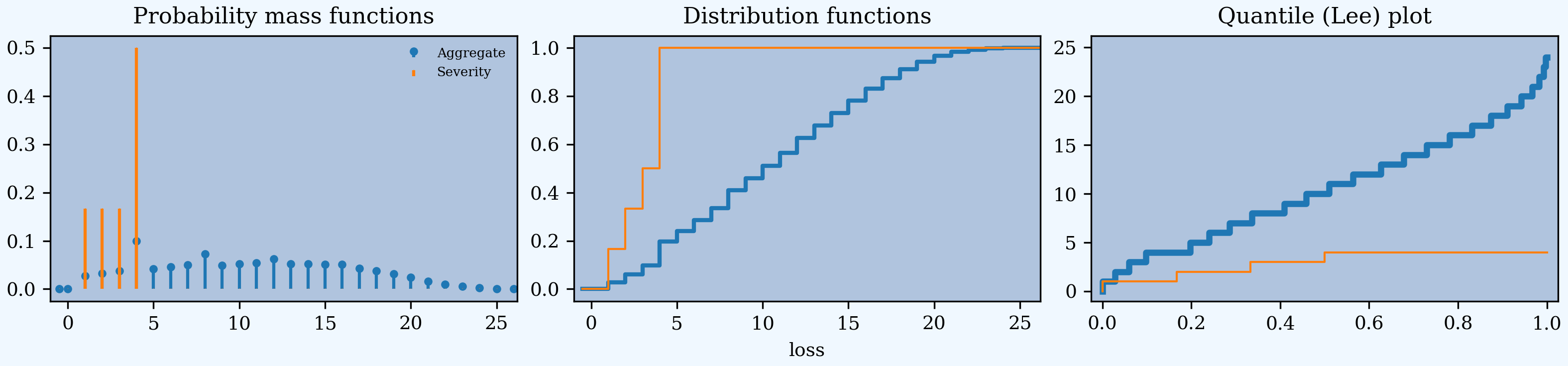
[1:6] is shorthand for [1,2,3,4,5,6]. The net severity equals 3 = (1 + 2 + 3 + 4 + 4 + 4) / 6.
The reinsurance_audit_df dataframe shows unconditional (per ground up claim) severity statistics by layer. Multiply by the claim count a02.n to get layer loss picks. The severity, ex, equals (1 + 2) / 6 = 0.5 (first block). The expected loss to the layer equals 0.5 * 3.5 = 1.75 (second block).
In [10]: qd(a02.reinsurance_audit_df['ceded'])

                             ex     var      sd     cv    skew
kind share limit attach
occ  1.0   1.0   4.0    0.33333 0.22222  0.4714 1.4142 0.70711
                 5.0    0.16667 0.13889 0.37268 2.2361  1.7889
     all   inf   gup        0.5 0.58333 0.76376 1.5275  1.1223

In [11]: qd(a02.reinsurance_audit_df['ceded'], sparsify=False)

                             ex     var      sd     cv    skew
kind share limit attach
occ  1.0   1.0   4.0    0.33333 0.22222  0.4714 1.4142 0.70711
occ  1.0   1.0   5.0    0.16667 0.13889 0.37268 2.2361  1.7889
occ  all   inf   gup        0.5 0.58333 0.76376 1.5275  1.1223

In [12]: qd(a02.reinsurance_audit_df['ceded'][['ex']] * a02.n)

                             ex
kind share limit attach
occ  1.0   1.0   4.0     1.1667
                 5.0    0.58333
     all   inf   gup       1.75
The reinsurance_occ_layer_df shows conditional layer expected loss and CV of loss, along with expected counts by layer and layer severity. The expected count to 1 xs 4 equals 3.5 / 3, because there is a 1/3 chance the layer attaches.
In [13]: qd(a02.reinsurance_occ_layer_df, sparsify=False)

stat                    ex     ex      ex     cv      cv      cv      en severity      pct
view                 ceded    net subject  ceded     net subject   ceded    ceded    ceded
share limit attach
1.0   1.0   4.0     1.1667 11.083   12.25 1.4142 0.42433 0.48795  1.1667        1 0.095238
1.0   1.0   5.0    0.58333 11.667   12.25 2.2361 0.44721 0.48795 0.58333        1 0.047619
all   inf   gup       1.75   10.5   12.25 1.5275  0.3849 0.48795     3.5      0.5  0.14286
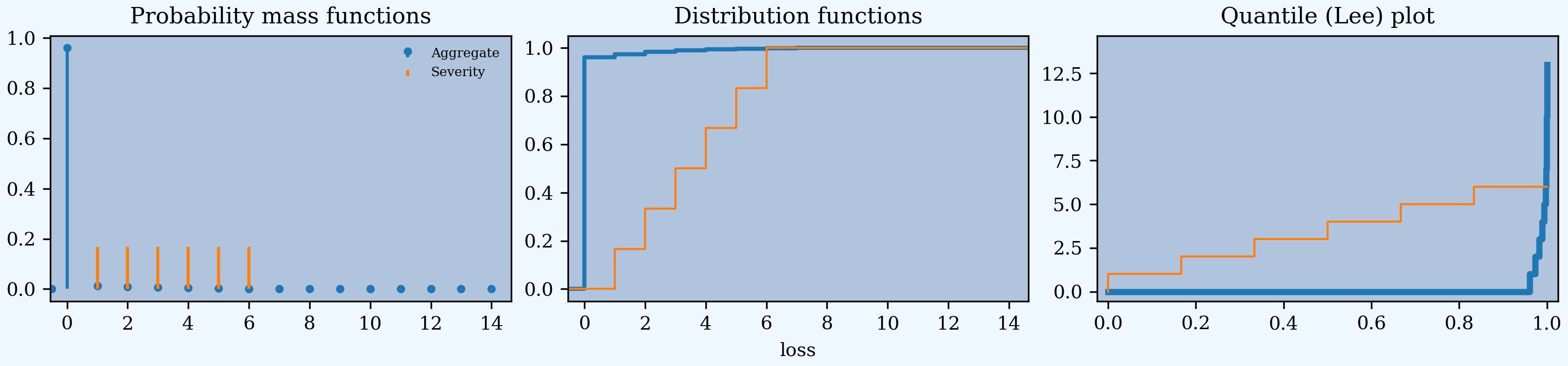
An aggregate excess of loss reinsurance layer, 12 xs 24, is specified after the frequency clause (you need to know frequency):
aggregate ceded to 12 xs 34.
Requesting ceded to propagates the ceded losses through to the aggregate. Refer to agg.Re:01 by name as a shorthand. reinsurance_audit_df reports expected loss to the aggregate layer. The layer is shown in two parts to illustrate reporting.
In [14]: a03 = build('agg Re:03 agg.Re:01 '
   ....:              'aggregate ceded to 6 xs 24 and 6 xs 30')
   ....:

In [15]: a03.plot()

In [16]: qd(a03)

      E[X] Est E[X] Err E[X]   CV(X) Est CV(X)  Skew(X) Est Skew(X)
X
Freq   3.5                   0.48795                  0
Sev    3.5      3.5        0 0.48795   0.48795        0  2.8529e-15
Agg  12.25  0.10661  -0.9913 0.55328    5.9383  0.28689      7.6018
log2 = 7, bandwidth = 1, validation: n/a, reinsurance.

In [17]: qd(a03.reinsurance_audit_df.stack(0))

                                       ex       var       sd      cv    skew
kind share limit attach
agg  1.0   6.0   24.0   ceded     0.10378   0.36108   0.6009  5.7901  6.9432
                        net        12.146    43.082   6.5637 0.54039 0.15351
                        subject     12.25    45.938   6.7777 0.55328 0.28689
                 30.0   ceded   0.0028292 0.0063577 0.079735  28.183  35.705
                        net        12.247    45.831   6.7698 0.55277 0.27937
                        subject     12.25    45.938   6.7777 0.55328 0.28689
     all   inf   gup    ceded     0.10661    0.4008  0.63309  5.9383  7.6018
                        net        12.143    43.009   6.5581 0.54005  0.1501
                        subject     12.25    45.938   6.7777 0.55328 0.28689
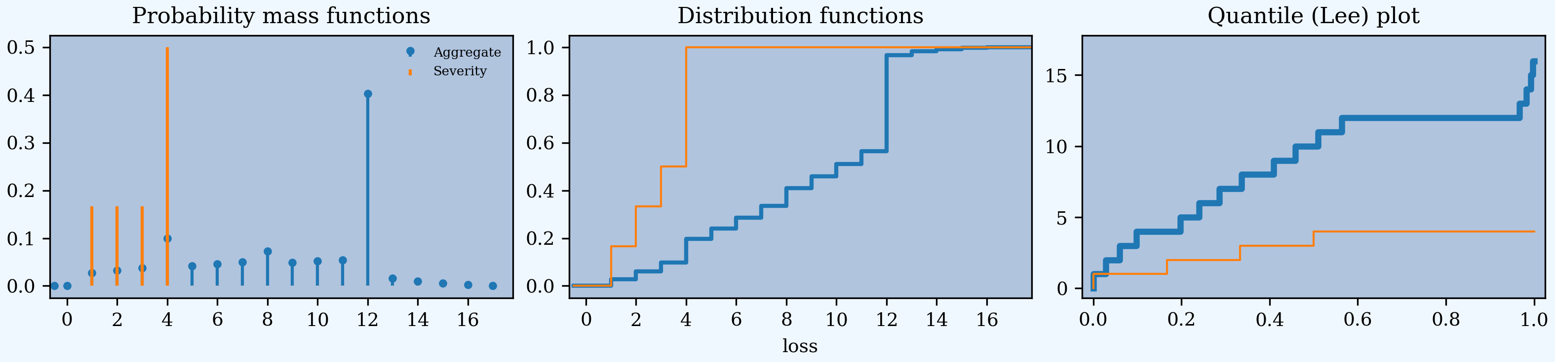
Occurrence and aggregate programs can both be applied. The ceded to and net of clauses can be mixed. You cannot refer to agg.Re:01 by name because you need to see into the object to apply the occurrence reinsurance.
In [18]: a04 = build('agg Re:04 dfreq [1:6] dsev [1:6] '
   ....:              'occurrence net of 1 xs 4 and 1 xs 5 '
   ....:              'aggregate net of 4 xs 12 and 4 xs 16')
   ....:

In [19]: a04.plot()

In [20]: qd(a04)

      E[X] Est E[X] Err E[X]   CV(X) Est CV(X)  Skew(X) Est Skew(X)
X
Freq   3.5                   0.48795                  0
Sev    3.5        3 -0.14286 0.48795    0.3849        0    -0.64952
Agg  12.25   8.8731 -0.27566 0.55328   0.41047  0.28689    -0.61588
log2 = 7, bandwidth = 1, validation: n/a, reinsurance.

In [21]: qd(a04.reinsurance_audit_df['ceded'])

                             ex     var      sd     cv    skew
kind share limit attach
occ  1.0   1.0   4.0    0.33333 0.22222  0.4714 1.4142 0.70711
                 5.0    0.16667 0.13889 0.37268 2.2361  1.7889
     all   inf   gup        0.5 0.58333 0.76376 1.5275  1.1223
agg  1.0   4.0   12.0     1.186  2.8219  1.6798 1.4164 0.88095
                 16.0   0.44087  1.1991   1.095 2.4838  2.4346
     all   inf   gup     1.6269  6.5022  2.5499 1.5674  1.3628
Layers can be specified as a share of or part of to account for coinsurance (partial placement) of the layer:
0.5 so 2 xs 2, read 50% share of 2 xs 2, or1 po 4 xs 10, read 1 part of 4 xs 10.
Warning
aggregate works with discrete distributions. All outcomes are multiples of the bucket size, bs. Any cession is rounded to a multiple of bs. Ensure bs is appropriate to capture cessions when applying share or part of. By default build uses bs=1 when it detects a discrete distribution, such as the die roll example. Ceding to 0.5 so 2 xs 2 produces ceded losses of 0.5 and net losses of 2.5. To capture these needs a much smaller discretization grid. Non-discrete aggregates plot as though they are continuous or mixed distributions.
These concepts are illustrated in the next example. Note the bucket size.
In [22]: a05 = build('agg Re:05 '
   ....:             'dfreq [1:6] dsev [1:6] '
   ....:             'occurrence net of 0.5 so 2 xs 2 and 2 xs 4 '
   ....:             'aggregate net of 1 po 4 xs 10 '
   ....:             , bs=1/512, log2=16)
   ....:

In [23]: a05.plot()

In [24]: qd(a05)

      E[X] Est E[X] Err E[X]   CV(X) Est CV(X)  Skew(X) Est Skew(X)
X
Freq   3.5                   0.48795                  0
Sev    3.5   2.4167 -0.30952 0.48795   0.30258        0    -0.98865
Agg  12.25   8.2063  -0.3301 0.55328   0.49122  0.28689   0.0035585
log2 = 16, bandwidth = 1/512, validation: n/a, reinsurance.

In [25]: qd(a05.reinsurance_audit_df['ceded'])

                             ex     var      sd      cv     skew
kind share limit attach
occ  0.5   2.0   2.0    0.58333 0.20139 0.44876 0.76931 -0.33297
     1.0   2.0   4.0        0.5 0.58333 0.76376  1.5275   1.1223
     all   inf   gup     1.0833  1.2014  1.0961  1.0118  0.64163
agg  0.25  4.0   10.0   0.25202 0.14516 0.38099  1.5117   1.1168
     all   inf   gup    0.25202 0.14516 0.38099  1.5117   1.1168

A tower of limits can be specified by giving the attachment points of each layer. The shorthand:
occurrence ceded to tower [0 1 2 5 10 20 36]
is equivalent to:
occurrence ceded to 1 xs 0 and 1 xs 1 and 3 xs 2 \
and 5 xs 5 and 10 xs 10 and 16 xs 20
Here is a summary of these examples. The audit dataframe gives a layering of aggregate losses. The plot is omitted; it is identical to gross since the tower covers all losses.
In [26]: a06 = build('agg Re:06 '
   ....:             'agg.Re:01 '
   ....:             'aggregate ceded to tower [0 1 2 5 10 20 36]')
   ....:

In [27]: a06.plot()

In [28]: qd(a06)

      E[X] Est E[X]   Err E[X]   CV(X) Est CV(X)  Skew(X) Est Skew(X)
X
Freq   3.5                     0.48795                  0
Sev    3.5      3.5          0 0.48795   0.48795        0  2.8529e-15
Agg  12.25    12.25 2.2204e-16 0.55328   0.55328  0.28689     0.28689
log2 = 7, bandwidth = 1, validation: n/a, reinsurance.

In [29]: qd(a06.reinsurance_audit_df['ceded'], sparsify=False)

                             ex        var         sd         cv        skew
kind share limit attach
agg  1.0   1.0   0.0          1 4.4409e-16 2.1073e-08 2.1073e-08 -4.7453e+07
agg  1.0   1.0   1.0    0.97222   0.027006    0.16434    0.16903      -5.747
agg  1.0   3.0   2.0     2.6997    0.64684    0.80426    0.29791     -2.6177
agg  1.0   5.0   5.0     3.5291     4.2422     2.0597    0.58361    -0.87928
agg  1.0   10.0  10.0     3.573     15.609     3.9508     1.1057     0.56831
agg  1.0   16.0  20.0   0.47593     2.2625     1.5042     3.1604      3.8783
agg  all   inf   gup      12.25     45.938     6.7777    0.55328     0.28689
See Reinsurance Functions for more about the reinsurance functions.
2.6.3. Modes of Reinsurance Analysis
Inwards reinsurance pricing is begins with an estimated loss pick, possibly supplemented by distribution and volatility statistics such as loss standard deviation or quantiles. aggregate can help in two ways.
Excess of loss exposure rating that accounts for the limits profile of the underlying business and how it interacts with excess layers. Uses only the severity distribution through difference of increased limits factors. This application is peripheral to the underlying purpose of
aggregate, but is very convenient nonetheless.The impact of treaty variable features that are derived from the full aggregate distribution of ceded losses and expenses—a showcase application.
Outwards reinsurance is evaluated based on the loss pick and the impact of the cession on the distribution of retained losses. Ceded re and broker actuaries often want the full gross and net outcome distributions.
2.6.4. Reinsurance Functions
This section demonstrates Aggregate methods and properties for reinsurance analysis. These are:
reinsurance_kinds()a text description of the kinds (occurrence and/or aggregate) of reinsurance applied.reinsurance_description()a text description of the layers and shares, by kind.reinsurance_occ_plot()plots subject (usually gross), ceded, and net severity, and aggregates created from each. Does not consider aggregate reinsurance.reinsurance_audit_dfdataframe summary by ceded, net, and subject, showing mean, CV, SD, and skewness of occurrence loss by layer and in total by kind.reinsurance_occ_layer_dfdataframe showing an expected loss layering analysis for occurrence reinsurance.reinsurance_dfdataframe showing all possible densities.reinsurance_report_dfdataframe showing mean, CV, skew, and SD statistics for each column inreinsurance_df.
These are illustrated using the a more realistic example that includes occurrence and aggregate reinsurance. Notice that the occurrence program just layers gross (subject) losses. Gross losses are then passed through to the aggregate program. This is done to illustrate the functions below. In a real-world application is is likely the bottom few occurrence layers would be dropped and you would pass the net of through to the aggregate.
In [30]: from aggregate import build, qd

In [31]: a = build('agg ReTester '
   ....:           '10 claims '
   ....:           '5000 xs 0 '
   ....:           'sev lognorm 100 cv 5 '
   ....:           'occurrence ceded to 250 xs 0 and 250 xs 250 and 500 xs 500 and 1000 xs 1000 and 3000 xs 2000 '
   ....:           'poisson '
   ....:           'aggregate ceded to 250 xs 750 and 1500 xs 1000 '
   ....:          )
   ....:

In [32]: qd(a)

       E[X] Est E[X]    Err E[X]   CV(X) Est CV(X)  Skew(X) Est Skew(X)
X
Freq     10                      0.31623            0.31623
Sev  95.058   95.057 -2.0186e-06  3.2307    3.2307   9.4329      9.4329
Agg  950.58    310.2    -0.67367  1.0695    1.7183   2.8646      1.7399
log2 = 16, bandwidth = 1/2, validation: n/a, reinsurance.

In [33]: print(a.reinsurance_kinds())
Occurrence and aggregate

In [34]: print(a.reinsurance_description())
Ceded to 100% share of 250 xs 0 and 100% share of 250 xs 250 and 100% share of 500 xs 500 and 100% share of 1,000 xs 1,000 and 100% share of 3,000 xs 2,000 per occurrence then ceded to 100% share of 250 xs 750 and 100% share of 1,500 xs 1,000 in the aggregate.
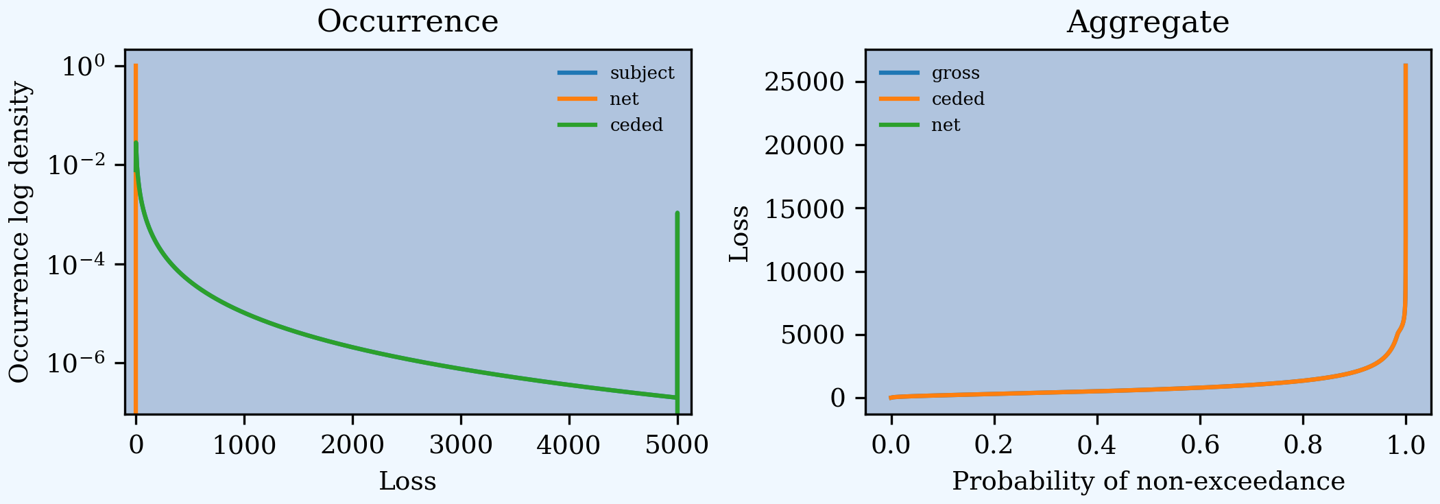
'plot shows the impact of occurrence reinsurance on severity and aggregate losses, and the ceded severity and aggregate.
In [35]: a.reinsurance_occ_plot()
The reinsurance_audit_df dataframe shows unconditional layer severity that “adds-up” to the total layer severity; compare to the total with the severity statistics in description above. These only match when the reinsurance layers exhaust the ground-up limit.
In [36]: qd(a.reinsurance_audit_df, sparsify=False)

                          ceded      ceded  ceded  ceded   ceded    net        net    net     net  \
                             ex        var     sd     cv    skew     ex        var     sd      cv
kind share limit  attach
occ  1.0   250.0  0.0    54.459     5603.2 74.854 1.3745  1.6845 40.599      72833 269.88  6.6474
occ  1.0   250.0  250.0  13.305     2720.7  52.16 3.9204  3.9945 81.753      73469 271.05  3.3155
occ  1.0   500.0  500.0  11.481     4748.2 68.907 6.0018  6.3905 83.576      64191 253.36  3.0315
occ  1.0   1000.0 1000.0 8.7092     7140.4 84.501 9.7025  10.609 86.348      57052 238.86  2.7662
occ  1.0   3000.0 2000.0 7.1035      15770 125.58 17.678  20.596 87.954      51379 226.67  2.5771
occ  all   inf    gup    95.057      94314 307.11 3.2307  9.4329      0          0      0     NaN
agg  1.0   250.0  750.0  89.854      13133  114.6 1.2754 0.58829 860.72 8.8125e+05 938.75  1.0907
agg  1.0   1500.0 1000.0 220.35  2.004e+05 447.67 2.0316  2.0217 730.22 4.2122e+05 649.02 0.88879
agg  all   inf    gup     310.2 2.8411e+05 533.02 1.7183  1.7399 640.37 3.3956e+05 582.72 0.90997

                            net subject    subject subject subject subject
                           skew      ex        var      sd      cv    skew
kind share limit  attach
occ  1.0   250.0  0.0    11.537  95.057      94314  307.11  3.2307  9.4329
occ  1.0   250.0  250.0   10.96  95.057      94314  307.11  3.2307  9.4329
occ  1.0   500.0  500.0   10.74  95.057      94314  307.11  3.2307  9.4329
occ  1.0   1000.0 1000.0 8.7905  95.057      94314  307.11  3.2307  9.4329
occ  1.0   3000.0 2000.0 5.6194  95.057      94314  307.11  3.2307  9.4329
occ  all   inf    gup       NaN  95.057      94314  307.11  3.2307  9.4329
agg  1.0   250.0  750.0   3.242  950.57 1.0335e+06  1016.6  1.0695  2.8646
agg  1.0   1500.0 1000.0 3.9477  950.57 1.0335e+06  1016.6  1.0695  2.8646
agg  all   inf    gup    4.8085  950.57 1.0335e+06  1016.6  1.0695  2.8646
The reinsurance_occ_layer_df dataframe shows unconditional aggregate statistics. The blocks ex and cv show values from audit_df times expected claim counts; en shows claim counts by layer. severity shows the implied conditional layer severity, equal to expected loss from audit_df divided by the probability of attaching the layer.
In [37]: qd(a.reinsurance_occ_layer_df, sparsify=False)

stat                    ex     ex      ex     cv     cv      cv       en severity      pct
view                 ceded    net subject  ceded    net subject    ceded    ceded    ceded
share limit  attach
1.0   250.0  0.0    544.59 405.99  950.57 1.3745 6.6474  3.2307       10   54.459   0.5729
1.0   250.0  250.0  133.05 817.53  950.57 3.9204 3.3155  3.2307  0.79248   167.89  0.13997
1.0   500.0  500.0  114.81 835.76  950.57 6.0018 3.0315  3.2307  0.36394   315.47  0.12078
1.0   1000.0 1000.0 87.092 863.48  950.57 9.7025 2.7662  3.2307  0.14697   592.59  0.09162
1.0   3000.0 2000.0 71.035 879.54  950.57 17.678 2.5771  3.2307 0.052009   1365.8 0.074729
all   inf    gup    950.57      0  950.57 3.2307    NaN  3.2307       10   95.057        1
The reinsurance_df density dataframe shows subject, ceded, and net occurrence (severity); aggregates created from each (without aggregate reinsurance); and subject, ceded, and net of requested aggregate reinsurance.
In [38]: qd(a.reinsurance_df, max_rows=20)

         loss  p_sev_gross  p_sev_ceded  p_sev_net  p_agg_gross_occ  p_agg_ceded_occ  \
loss
0.0         0    0.0078283    0.0078283          1       4.9097e-05       4.9097e-05
0.5       0.5     0.027461     0.027461          0       1.3482e-05       1.3482e-05
1.0         1     0.028318     0.028318          0       1.5754e-05       1.5754e-05
1.5       1.5     0.026716     0.026716          0       1.7104e-05       1.7104e-05
2.0         2     0.024836     0.024836          0         1.83e-05         1.83e-05
2.5       2.5     0.023058     0.023058          0       1.9467e-05       1.9467e-05
3.0         3     0.021453     0.021453          0       2.0635e-05       2.0635e-05
3.5       3.5     0.020023     0.020023          0       2.1812e-05       2.1812e-05
4.0         4      0.01875      0.01875          0          2.3e-05          2.3e-05
4.5       4.5     0.017615     0.017615          0         2.42e-05         2.42e-05
...       ...          ...          ...        ...              ...              ...
32763.0 32763            0            0          0                0                0
32763.5 32764            0            0          0                0                0
32764.0 32764            0            0          0                0                0
32764.5 32764            0            0          0                0                0
32765.0 32765            0            0          0                0                0
32765.5 32766            0            0          0                0                0
32766.0 32766            0            0          0                0                0
32766.5 32766            0            0          0                0                0
32767.0 32767            0            0          0                0                0
32767.5 32768            0            0          0                0                0

         p_agg_net_occ  p_agg_gross  p_agg_ceded  p_agg_net
loss
0.0                  1   4.9097e-05      0.57612 4.9097e-05
0.5                  0   1.3482e-05   0.00029446 1.3482e-05
1.0                  0   1.5754e-05   0.00029422 1.5754e-05
1.5                  0   1.7104e-05   0.00029398 1.7104e-05
2.0                  0     1.83e-05   0.00029374   1.83e-05
2.5                  0   1.9467e-05   0.00029351 1.9467e-05
3.0                  0   2.0635e-05   0.00029327 2.0635e-05
3.5                  0   2.1812e-05   0.00029303 2.1812e-05
4.0                  0      2.3e-05   0.00029279    2.3e-05
4.5                  0     2.42e-05   0.00029256   2.42e-05
...                ...          ...          ...        ...
32763.0              0   4.5631e-19            0          0
32763.5              0    4.471e-19            0          0
32764.0              0   4.6061e-19            0          0
32764.5              0   4.5894e-19            0          0
32765.0              0   4.3986e-19            0          0
32765.5              0   4.4694e-19            0          0
32766.0              0   4.4323e-19            0          0
32766.5              0   4.3824e-19            0          0
32767.0              0   4.3557e-19            0          0
32767.5              0   4.4901e-19            0          0
The reinsurance_report_df shows statistics for the densities in reinsurance_df. The p_agg_gross column matches the theoretical (gross) output shown in qd(a) at the top and the p_agg_ceded column matches the estimated output because the aggregate program requested ceded to output. The net column is the difference.
In [39]: qd(a.reinsurance_report_df)

      p_sev_gross  p_sev_ceded  p_sev_net  p_agg_gross_occ  p_agg_ceded_occ  p_agg_net_occ  \
mean       95.057       95.057          0           950.57           950.57              0
cv         3.2307       3.2307        NaN           1.0695           1.0695            NaN
sd         307.11       307.11        NaN           1016.6           1016.6            NaN
skew       9.4329       9.4329        NaN           2.8646           2.8646            NaN

      p_agg_gross  p_agg_ceded  p_agg_net
mean       950.57        310.2     640.37
cv         1.0695       1.7183    0.90997
sd         1016.6       533.02     582.72
skew       2.8646       1.7399     4.8085
2.6.5. Casualty Exposure Rating
This example calculates the loss pick for excess layers across a subject portfolio with different underlying limits and deductibles but a common severity curve. The limit profile is given by a premium distribution and the expected loss ratio varies by limit. Values are in 000s. Policies at 1M and 2M limits are ground-up and those at 5M and 10M limits have a 100K and 250K deductible. The full assumptions are:
In [40]: profile = pd.DataFrame({'limit': [1000, 2000, 5000, 10000],
   ....:                         'ded'  : [0, 0, 100, 250],
   ....:                         'premium': [10000, 5000, 2500, 1500],
   ....:                         'lr': [.75, .75, .7, .65]
   ....:                        }, index=pd.Index(range(4), name='class'))
   ....:

In [41]: qd(profile)

       limit  ded  premium   lr
class
0       1000    0    10000 0.75
1       2000    0     5000 0.75
2       5000  100     2500  0.7
3      10000  250     1500 0.65
The severity is a lognormal with an unlimited mean of 50 and cv of 10, \(\sigma=2.148\).
The gross portfolio and tower are created in a07.
A typical XOL tower up to 10M is created by specifying the layer break points in an occurrence ceded to tower clause.
In [42]: a07 = build('agg Re:07 '
   ....:            f'{profile.premium.values} premium at {profile.lr.values} lr '
   ....:            f'{profile.limit.values} xs {profile.ded.values} '
   ....:             'sev lognorm 50 cv 10 '
   ....:             'occurrence ceded to tower [0 250 500 1000 2000 5000 10000] '
   ....:             'poisson '
   ....:             , approximation='exact', log2=18, bs=1/2)
   ....:

In [43]: qd(a07)

       E[X] Est E[X]    Err E[X]    CV(X) Est CV(X)  Skew(X) Est Skew(X)
X
Freq 292.72                      0.058448           0.058448
Sev  47.741   47.737 -8.6055e-05   4.0096      4.01   15.901      15.901
Agg   13975    13974 -8.6055e-05  0.24153   0.24156  0.88974     0.88974
log2 = 18, bandwidth = 1/2, validation: n/a, reinsurance.
There are special options in build because the claim count is high: 292.7. To force a convolution use approximation='exact'. Reviewing the default bs=1/2 and log2=16 shows a moderate error. Looking at the density via:
a07.density_df.p_total.plot(logy=True)
shows aliasing, i.e., there is not enough space in the answer. Adjust by increasing log2 from 16 to 18 and leaving bs=1/2.
The dataframe reinsurance_occ_layer_df shows layer expected loss, CV, counts, and conditional severity. The last column shows the percent of subject ceded to each layer.
In [44]: qd(a07.reinsurance_occ_layer_df, sparsify=False)

stat                    ex          ex      ex     cv     cv      cv       en severity       pct
view                 ceded         net subject  ceded    net subject    ceded    ceded     ceded
share limit  attach
1.0   250.0  0.0    8724.1      5249.7   13974 1.9905 8.8564    4.01   292.72   29.803   0.62432
1.0   250.0  250.0  2076.6       11897   13974 5.4793 4.0236    4.01   12.063   172.15   0.14861
1.0   500.0  500.0  1917.9       12056   13974 8.0564 3.7267    4.01   5.8545   327.58   0.13725
1.0   1000.0 1000.0 775.37       13198   13974 17.887 3.5805    4.01   1.2306    630.1  0.055488
1.0   3000.0 2000.0 400.74       13573   13974 41.327  3.509    4.01  0.26392   1518.4  0.028678
1.0   5000.0 5000.0  79.06       13895   13974 122.64 3.8196    4.01 0.027983   2825.3 0.0056577
all   inf    gup     13974 -7.8694e-09   13974   4.01    NaN    4.01   292.72   47.737         1
2.6.6. Property Risk Exposure Rating
Property risk exposure rating differs from casualty in part because the severity distribution varies with each risk (location). Rather than a single ground-up severity curve per class, there is a size of loss distribution normalized by property total insured value (TIV).
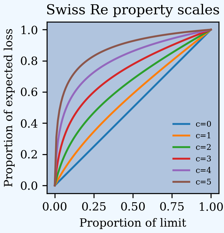
We start by introducing the Swiss Re severity curves, Bernegger [1997] using a moments-matched beta distribution. The function G defines the MBBEFD distribution, parameterized by c.
In [45]: from aggregate import xsden_to_meancv

In [46]: import scipy.stats as ss

In [47]: import numpy as np

In [48]: import matplotlib.pyplot as plt

In [49]: def bb(c):
   ....:     return np.exp(3.1 - 0.15*c*(1+c))
   ....:

In [50]: def bg(c):
   ....:     return np.exp((0.78 + 0.12*c)*c)
   ....:

In [51]: def G(x, c):
   ....:     b = bb(c)
   ....:     g = bg(c)
   ....:     return np.log(((g - 1) * b + (1 - g * b) * b**x) / (1 - b)) / np.log(g * b)
   ....:
Here are the base curves, compare Figure 4.2 in Bernegger [1997]. The curve c=5 is close to the Lloyd’s curve (scale).
In [52]: fig, ax = plt.subplots(1, 1, figsize=(2.45, 2.55), constrained_layout=True)

In [53]: ans = []

In [54]: ps = np.linspace(0,1,101)

In [55]: for c in [0, 1, 2, 3, 4, 5]:
   ....:     gs = G(ps, c)
   ....:     ax.plot(ps, gs, label=f'c={c}')
   ....:     ans.append([c, *xsden_to_meancv(ps[1:], np.diff(gs))])
   ....:

In [56]: ax.legend(loc='lower right');

In [57]: ax.set(xlabel='Proportion of limit', ylabel='Proportion of expected loss',
   ....:        title='Swiss Re property scales');
   ....:
Next, approximate these curves with a beta distribution to make them easier for us to use in aggregate. Here are the parameters and fit graphs for each curve.
In [58]: swiss = pd.DataFrame(ans, columns=['c', 'mean', 'cv'])

In [59]: def beta_ab(m, cv):
   ....:     v = (m * cv) ** 2
   ....:     sev_a = m * (m * (1 - m) / v - 1)
   ....:     sev_b = (1 - m) * (m * (1 - m) / v - 1)
   ....:     return sev_a, sev_b
   ....:

In [60]: a, b = beta_ab(swiss['mean'], swiss.cv)

In [61]: swiss['a'] = a

In [62]: swiss['b'] = b

In [63]: swiss = swiss.set_index('c')

In [64]: qd(swiss)

     mean      cv       a      b
c
0   0.505 0.57161    1.01   0.99
1 0.44108 0.67278 0.79375 1.0058
2 0.36415 0.81654 0.58953 1.0294
3 0.28003  1.0103 0.42538 1.0937
4 0.19858  1.2531 0.31176 1.2582
5 0.13101  1.5171 0.24654 1.6353

In [65]: fig, axs = plt.subplots(2, 3, figsize=(3 * 2.45, 2 * 2.45), constrained_layout=True)

In [66]: for ax, (c, r) in zip(axs.flat, swiss.iterrows()):
   ....:     gs = G(ps, c)
   ....:     fz = ss.beta(r.a, r.b)
   ....:     ax.plot(ps, gs, label=f'c={c}')
   ....:     ax.plot(ps, fz.cdf(ps), label=f'beta fit')
   ....:     ans.append([c, *xsden_to_meancv(ps[1:], np.diff(gs))])
   ....:     ax.legend(loc='lower right');
   ....:

In [67]: fig.suptitle('Beta approximations to Swiss Re property curves');

Work on a property schedule with the following TIVs and deductibles. The premium rate is 0.35 per 100 and the loss ratio is 55%.
In [68]: schedule = pd.DataFrame({
   ....:     'locid': range(10),
   ....:     'tiv': [850, 950, 1250, 1500, 4500, 8000, 9000, 12000, 25000, 50000],
   ....:     'ded': [ 10,  10,   20,   20,   50,   100, 500,  1000,  5000,  5000]}
   ....:     ).set_index('locid')
   ....:

In [69]: schedule['premium'] = schedule.tiv / 100 * 0.35

In [70]: schedule['lr'] = 0.55

In [71]: qd(schedule)

         tiv   ded  premium   lr
locid
0        850    10    2.975 0.55
1        950    10    3.325 0.55
2       1250    20    4.375 0.55
3       1500    20     5.25 0.55
4       4500    50    15.75 0.55
5       8000   100       28 0.55
6       9000   500     31.5 0.55
7      12000  1000       42 0.55
8      25000  5000     87.5 0.55
9      50000  5000      175 0.55
Build the stochastic model using a Swiss Re c=3 scale. Use a gamma mixed Poisson frequency with a CV of 3 to reflect the potential for catastrophe losses. Use a tower clause to set up the analysis of a per risk tower. Increase bs to 2 based on high error with recommended bs=1.
In [72]: beta_a, beta_b = swiss.loc[3, ['a', 'b']]

In [73]: a08 = build('agg Re:08 '
   ....:            f'{schedule.premium.values} premium at {schedule.lr.values} lr '
   ....:            f'{schedule.tiv.values} xs {schedule.ded.values} '
   ....:            f'sev {schedule.tiv.values} * beta {beta_a} {beta_b} ! '
   ....:             'occurrence ceded to tower [0 1000 5000 10000 20000 inf] '
   ....:             'mixed gamma 2 '
   ....:             , bs=2)
   ....:

In [74]: qd(a08)

         E[X] Est E[X]    Err E[X]  CV(X) Est CV(X)  Skew(X) Est Skew(X)
X
Freq 0.081693                        4.03             5.0226
Sev    2663.9   2663.9 -1.2094e-07 2.2311    2.2311   3.8455      3.8455
Agg    217.62   217.62 -1.3778e-07 8.7849    8.7849   14.303      14.303
log2 = 16, bandwidth = 2, validation: n/a, reinsurance.
The shared mixing increases the frequency and aggregate CV and skewness.
In [75]: qd(a08.report_df.loc[
   ....:     ['freq_m', 'freq_cv', 'freq_skew', 'agg_cv', 'agg_skew'],
   ....:     ['independent', 'mixed']])
   ....:

view      independent    mixed
statistic
freq_m       0.081693 0.081693
freq_cv        3.5576     4.03
freq_skew      3.6749   5.0226
agg_cv         8.6169   8.7849
agg_skew       14.248   14.303
Look at reinsurance_occ_layer_df to summarize the analysis.
In [76]: qd(a08.reinsurance_occ_layer_df, sparsify=False)

stat                      ex     ex      ex      cv     cv      cv        en severity     pct
view                   ceded    net subject   ceded    net subject     ceded    ceded   ceded
share limit   attach
1.0   1000.0  0.0     38.473 179.15  217.62 0.93539  2.612  2.2311   0.05879   654.41 0.17679
1.0   4000.0  1000.0  74.293 143.33  217.62  1.6859 2.7968  2.2311  0.027946   2658.4 0.34139
1.0   5000.0  5000.0  43.156 174.47  217.62  2.6872 2.2324  2.2311  0.012623   3418.8 0.19831
1.0   10000.0 10000.0 37.782 179.84  217.62  4.1476 1.9578  2.2311 0.0059027   6400.9 0.17362
1.0   inf     20000.0 23.917  193.7  217.62  7.2389   1.91  2.2311 0.0021465    11143  0.1099
all   inf     gup     217.62      0  217.62  2.2311    NaN  2.2311  0.081693   2663.9       1
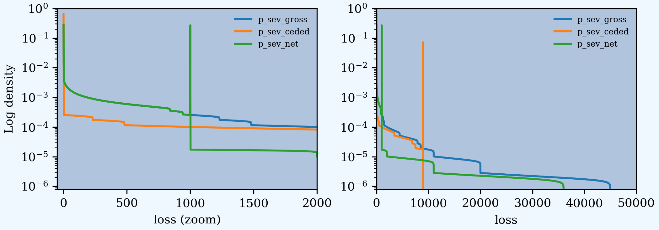
Add plots of gross, ceded, and net severity with the placed program, 4000 xs 1000 and 5000 xs 5000. (The net is zero with the tower clause, so we have to recompute.) The left and right plots differ only in the x-axis scale.
In [77]: a09 = build('agg Re:09 '
   ....:            f'{schedule.premium.values} premium at {schedule.lr.values} lr '
   ....:            f'{schedule.tiv.values} xs {schedule.ded.values} '
   ....:            f'sev {schedule.tiv.values} * beta {beta_a} {beta_b} ! '
   ....:             'occurrence ceded to 4000 xs 1000 and 5000 xs 5000 '
   ....:             'mixed gamma 2 ', bs=2)
   ....:

In [78]: qd(a09)

         E[X] Est E[X] Err E[X]  CV(X) Est CV(X)  Skew(X) Est Skew(X)
X
Freq 0.081693                     4.03             5.0226
Sev    2663.9   1437.7 -0.46031 2.2311    1.9215   3.8455      1.8785
Agg    217.62   117.45 -0.46031 8.7849     7.838   14.303      9.4024
log2 = 16, bandwidth = 2, validation: n/a, reinsurance.

In [79]: fig, axs = plt.subplots(1, 2, figsize=(2 * 3.5, 2.45), constrained_layout=True); \
   ....: ax0, ax1 = axs.flat; \
   ....: df = a09.reinsurance_df; \
   ....: df.filter(regex='sev_[gcn]').plot(logy=True, xlim=[-50, 2000], ylim=[0.8e-6, 1] , ax=ax0); \
   ....: df.filter(regex='sev_[gcn]').plot(logy=True, xlim=[0, 50000], ylim=[0.8e-6, 1], ax=ax1); \
   ....: ax0.set(xlabel='loss (zoom)', ylabel='Log density');
   ....:

In [80]: ax1.set(xlabel='loss', ylabel='');
And finally, plot the corresponding aggregate distributions.
In [81]: fig, axs = plt.subplots(2, 2, figsize=(2 * 3.5, 2 * 2.45), constrained_layout=True); \
   ....: ax0, ax1, ax2, ax3 = axs.flat; \
   ....: df.filter(regex='agg_.*_occ').plot(logy=True, xlim=[-50, 2000], ylim=[0.8e-6, 1] , ax=ax0); \
   ....: (1 - df.filter(regex='agg_.*_occ').cumsum()).plot(logy=True, xlim=[-50, 2000], ylim=[1e-3, 1], ax=ax2); \
   ....: df.filter(regex='agg_.*_occ').plot(logy=True, xlim=[0, 50000], ylim=[0.8e-12, 1], ax=ax1); \
   ....: (1 - df.filter(regex='agg_.*_occ').cumsum()).plot(logy=True, xlim=[0, 50000], ylim=[1e-9, 1], ax=ax3); \
   ....: ax0.set(xlabel='', ylabel='Log density'); \
   ....: ax1.set(xlabel='', ylabel=''); \
   ....: ax2.set(xlabel='loss (zoom)', ylabel='Log survival');
   ....:

In [82]: ax3.set(xlabel='loss', ylabel='');

2.6.7. Variable Features
Reinsurance treaties can incorporate variable features that alter the contract cash flows. These can impact losses, premiums, or expenses (through the ceding commission). They can apply to quota share and excess treaties.
Variable features altering Loss cash flows
Aggregate limits and deductibles
Loss corridor
Limited reinstatements for excess treaties, by number of covered events or an aggregate limit
Variable features altering Premium cash flows
Swing or retro rating or margin-plus premium, where the premium equals losses times an expense factor subject to a maximum and minimum. See also Individual Risk Pricing.
Variable features altering Expense cash flows
Sliding scale commission
Profit commission or profit share
A loss corridor and sliding scale commission have a similar impact; both concentrate the impact of the treaty on tail outcomes. Aggregate features have the opposite effect; concentrating the impact on body outcomes and lowering effectiveness on tail outcomes.
Premium and expense related features are substitutes, the former used on treaties without ceding commissions.
2.6.8. Inwards Analysis of Bear and Nemlick Variable Features
Bear and Nemlick [1990] analyze six treaties with variable features across four portfolios.
These examples are included because they are realistic and show that aggregate produces the same answers as a published reference.
The subject losses defined as follows.
Treaty 1 and 4.
Cover: 160 xs 40
Subject business
Two classes
Subject premium 3000 and 6000
Loss rate 4% and 3%
Severity: single parameter Pareto with shape 0.9 and 0.95
Treaty 2 and 5.
Cover: 700 xs 300
Subject business
Three classes
Subject premium 2000 each
Loss rate 10%, 14%, 21%
Severity: single parameter Pareto with shape 1.5, 1.3, 1.1
Treaty 3.
Cover: 400 xs 100
Subject business
Three classes
Subject premium 4500, 4500, 1000
Loss rate 3.2%, 3.8%, 3.5%
Severity: single parameter Pareto with shape 1.1.
Treaty 6.
Cover: 900 xs 100
Subject business
Subject premium 25000
Layer loss cost 10% of subject premium
Portfolio CV 0.485
They include a variety of frequency assumptions, including Poisson, negative binomial with variance multiplier based on a gross multiplier of 2 or 3 adjusted for excess frequency, mixing variance 0.05 and 0.10. Excess counts get closer to Poisson and so the difference between the two is slight.
The next table shows Bear and Nemlick’s estimated premium rates.

Bear and Nemlick’s estimated premium rates by program by numerical method. The Lognormal Model column uses a method of moments fit to the aggregate mean and CV. The Collective Risk Model columns uses the Heckman-Meyers continuous FFT method.
Heckman and Meyers describe claim count contagion and frequency parameter uncertainty, which they model using a mixed-Poisson frequency distribution. Their parameter \(c\) is the variance of the mixing distribution. The value c=0.05 is replicated in DecL with the frequency clause mixed gamma 0.05**0.5, since DecL is based on the CV of the mixing distribution (the mean is always 1).
Heckman and Meyers also describe severity parameter uncertainty, which they model with an inverse gamma variable with mean 1 and variance \(b\). There is no analog of severity uncertainty in DecL. For finite excess layers it has a muted impact on results. Heckman and Meyers call \(c\) the contagion parameter and \(b\) the mixing parameter, which is confusing in our context. To approximate these columns use
c=0,b=0corresponds to the DecL frequency clausepoisson.c=0.05,b=...is close to DecL frequency clausemixed gamma 0.05**0.5.c=0.1,b=...is close to DecL frequency clausemixed gamma 0.1**0.5.
2.6.8.1. Specifying the Single Parameter Pareto
Losses to an excess layer specified by a single parameter Pareto are the same as losses to a ground-up layer with a shifted Pareto.
Example.
For 400 xs 100 and Pareto shape 1.1, these two DecL programs produce identical results:
4 claims 400 xs 100 sev 100 * pareto 1.1 poisson

4 claims 400 xs 0 sev 100 * pareto 1.1 - 100 poisson
2.6.8.2. Treaty 1: Aggregate Deductible
Treaty 1 adds an aggregate deductible of 360, equal to 3% of subject premium.
Setup the gross portfolio.
In [83]: import numpy as np

In [84]: from aggregate import build, mv, qd, xsden_to_meancvskew, \
   ....:      mu_sigma_from_mean_cv, lognorm_lev
   ....:

In [85]: mix_cv = ((1.036-1)/5.154)**.5; mix_cv
Out[85]: 0.08357551150546018

In [86]: a10 = build('agg Re:BN1 '
   ....:             '[9000 3000] exposure at [0.04 0.03] rate '
   ....:             '160 xs 0 '
   ....:             'sev 40 * pareto [0.9 0.95] - 40 '
   ....:            f'mixed gamma {mix_cv} ')
   ....:

In [87]: qd(a10)

       E[X] Est E[X]    Err E[X]   CV(X) Est CV(X)  Skew(X) Est Skew(X)
X
Freq 6.4966                      0.40114            0.41855
Sev  69.267   69.267 -1.2751e-08 0.87703   0.87703  0.50056     0.50056
Agg     450      450 -2.1418e-07  0.5285    0.5285  0.62441     0.62436
log2 = 16, bandwidth = 1/32, validation: fails agg mean error >> sev, possible aliasing; try larger bs.
The portfolio CV matches 0.528, reported in Bear and Nemlick Appendix F, Exhibit 1.
There are several ways to estimate the impact of the AAD on recovered losses.
By hand, adjust losses and use the distribution of outcomes from a.density_df. The last line computes the sum-product of losses net of AAD times probabilities, i.e., the expected loss cost.
In [88]: bit = a10.density_df[['loss', 'p_total']]

In [89]: bit['loss'] = np.maximum(0, bit.loss - 360)

In [90]: bit.prod(axis=1).sum()
Out[90]: np.float64(142.75712297665373)
More in the spirit of aggregate: create a new Aggregate applying the AAD using a DecL aggregate net of reinsurance clause. Alternatively use aggregate ceded to inf xs 360 (not shown).
In [91]: a11 = build('agg Re:BN1a '
   ....:             '[9000 3000] exposure at [0.04 0.03] rate '
   ....:             '160 xs 0 '
   ....:             'sev 40 * pareto [0.9 0.95] - 40 '
   ....:            f'mixed gamma {mix_cv} '
   ....:             'aggregate net of 360 xs 0 ')
   ....:

In [92]: qd(a11)

       E[X] Est E[X]    Err E[X]   CV(X) Est CV(X)  Skew(X) Est Skew(X)
X
Freq 6.4966                      0.40114            0.41855
Sev  69.267   69.267 -1.2751e-08 0.87703   0.87703  0.50056     0.50056
Agg     450   142.76    -0.68276  0.5285    1.2873  0.62441      1.5337
log2 = 16, bandwidth = 1/32, validation: n/a, reinsurance.

In [93]: gross = a11.agg_m; net = a11.est_m; ins_charge = net / gross

In [94]: net, ins_charge
Out[94]: (np.float64(142.75888602897442), np.float64(0.31724196895327644))
Bear and Nemlick use a lognormal approximation to the aggregate.
In [95]: mu, sigma = mu_sigma_from_mean_cv(a10.agg_m, a10.agg_cv)

In [96]: elim_approx = lognorm_lev(mu, sigma, 1, 360)

In [97]: a11.agg_m - elim_approx, 1 - elim_approx / a11.agg_m
Out[97]: (np.float64(132.0633321885802), np.float64(0.29347407153017824))
The lognormal overstates the value of the AAD, resulting in a lower net premium. This is because the approximating lognormal is much more skewed.
In [98]: fz = a11.approximate('lognorm')

In [99]: fz.stats('s'), a11.est_skew
Out[99]: (np.float64(5.995433538387627), np.float64(1.5337492513582904))
Bear and Nemlick report the Poisson approximation and a Heckman-Meyers convolution with mixing and contagion equal 0.05. We can compute the Poisson exactly and approximate Heckman-Meyers with contagion but no mixing. Changing 0.05 to 0.10 is close to the b=0.1 column.
In [100]: a12 = build('agg Re:BN1p '
   .....:             '[9000 3000] exposure at [0.04 0.03] rate '
   .....:             '160 xs 0 '
   .....:             'sev 40 * pareto [0.9 0.95] - 40 '
   .....:            f'poisson '
   .....:             'aggregate net of 360 xs 0 ')
   .....:

In [101]: qd(a12)

       E[X] Est E[X]    Err E[X]   CV(X) Est CV(X)  Skew(X) Est Skew(X)
X
Freq 6.4966                      0.39234            0.39234
Sev  69.267   69.267 -1.2751e-08 0.87703   0.87703  0.50056     0.50056
Agg     450    141.8    -0.68489 0.52185    1.2794  0.60775      1.5152
log2 = 16, bandwidth = 1/32, validation: n/a, reinsurance.

In [102]: a13 = build('agg Re:BN1c '
   .....:             '[9000 3000] exposure at [0.04 0.03] rate '
   .....:             '160 xs 0 '
   .....:             'sev 40 * pareto [0.9 0.95] - 40 '
   .....:             'mixed gamma 0.05**.5 '
   .....:             'aggregate net of 360 xs 0 ')
   .....:

In [103]: qd(a13)

       E[X] Est E[X]    Err E[X]   CV(X) Est CV(X)  Skew(X) Est Skew(X)
X
Freq 6.4966                      0.45158             0.5623
Sev  69.267   69.267 -5.1006e-08 0.87703   0.87703  0.50056     0.50056
Agg     450   148.41     -0.6702 0.56774    1.3332  0.72251      1.6412
log2 = 16, bandwidth = 1/16, validation: n/a, reinsurance.
Here is a summary of the different methods, compare Bear and Nemlick Table 1, row 1, page 75.
In [104]: bit = pd.DataFrame([a10.agg_m,
   .....:     a11.describe.iloc[-1, 1],
   .....:     a12.describe.iloc[-1, 1],
   .....:     a13.describe.iloc[-1, 1],
   .....:     a11.agg_m - elim_approx],
   .....:     columns=['Loss cost'],
   .....:     index=pd.Index(['Gross', 'NB', 'Poisson', 'c=0.05', 'lognorm'],
   .....:                   name='Method'))
   .....:

In [105]: bit['Premium'] = bit['Loss cost'] * 100 / 75

In [106]: bit['Rate'] = bit.Premium / 12000

In [107]: qd(bit, accuracy=5)

         Loss cost  Premium     Rate
Method
Gross          450      600     0.05
NB          142.76   190.35 0.015862
Poisson      141.8   189.07 0.015755
c=0.05      148.41   197.88  0.01649
lognorm     132.06   176.08 0.014674
2.6.8.3. Treaty 2: Aggregate Limit
Treaty 2 adds an aggregate limit of 2800, i.e., 3 full reinstatements plus the original limit.
Setup the gross portfolio.
In [108]: a14 = build('agg Re:BN2 '
   .....:             '[2000 2000 2000] exposure at [.1 .14 .21] rate '
   .....:             '700 xs 0 '
   .....:             'sev 300 * pareto [1.5 1.3 1.1] - 300 '
   .....:             'mixed gamma 0.07 '
   .....:             , bs=1/8)
   .....:

In [109]: qd(a14)

       E[X] Est E[X]    Err E[X]   CV(X) Est CV(X)  Skew(X) Est Skew(X)
X
Freq 2.8949                       0.5919            0.60017
Sev   310.9    310.9 -8.2604e-09 0.83714   0.83714  0.46335     0.46335
Agg     900      900 -8.4265e-09 0.76969   0.76969  0.90207     0.90207
log2 = 16, bandwidth = 1/8, validation: not unreasonable.
Specify bs=1/8 since the error was too high with the default bs=1/16.
The portfolio CV matches 0.770, reported in Bear and Nemlick Appendix G, Exhibit 1. The easiest way to value the aggregate limit to use an aggregate ceded to clause.
In [110]: a14n = build('agg Re:BN2a '
   .....:              '[2000 2000 2000] exposure at [.1 .14 .21] rate '
   .....:              '700 xs 0 '
   .....:              'sev 300 * pareto [1.5 1.3 1.1] - 300 '
   .....:              'mixed gamma 0.07 '
   .....:              'aggregate ceded to 2800 xs 0'
   .....:              , bs=1/8)
   .....:

In [111]: qd(a14n)

       E[X] Est E[X]    Err E[X]   CV(X) Est CV(X)  Skew(X) Est Skew(X)
X
Freq 2.8949                       0.5919            0.60017
Sev   310.9    310.9 -8.2604e-09 0.83714   0.83714  0.46335     0.46335
Agg     900   894.68  -0.0059104 0.76969    0.7544  0.90207     0.72143
log2 = 16, bandwidth = 1/8, validation: n/a, reinsurance.
Applying a 20% coinsurance and grossing up by 100/60 produces the premium and rate. Using Poisson frequency, or mixed gamma with mix \(\sqrt{0.05}\) or \(\sqrt{0.1}\) ties closely to Table I, row 2.
In [112]: p = a14n.est_m * (1 - 0.2) * 100 / 60

In [113]: p, p / 6000
Out[113]: (np.float64(1192.907570662762), np.float64(0.19881792844379367))
aggregate induces correlation between the three classes because they share mixing variables. The report_df shows the details by line and compares with an independent sum.
In [114]: qd(a14.report_df.iloc[:, :-2])

view             0       1       2 independent   mixed
statistic
name        Re:BN2  Re:BN2  Re:BN2      Re:BN2  Re:BN2
limit          700     700     700         700     700
attachment       0       0       0           0       0
el             200     280     420         900     900
freq_m     0.73701 0.92362  1.2342      2.8949  2.8949
freq_cv     1.1669  1.0429 0.90284     0.58919  0.5919
freq_skew   1.1711  1.0476 0.90827     0.59209 0.60017
sev_m       271.37  303.15   340.3       310.9   310.9
sev_cv      0.9087 0.84973 0.78339     0.83714 0.83714
sev_skew   0.72529 0.51332 0.27989     0.46335 0.46335
agg_m          200     280     420         900     900
agg_cv      1.5755  1.3672  1.1456     0.76767 0.76969
agg_skew    1.9025  1.6073  1.3121     0.89708 0.90207
2.6.8.4. Treaty 3: Loss Corridor
Treaty 3 is a loss corridor from expected layer losses to twice expected. The reinsurance pays up to expected and beyond twice expected.
Setup the gross portfolio with CV 0.905. Use a larger bs to reduce error.
In [115]: a15 = build('agg Re:BN3 '
   .....:             '[4500 4500 1000] exposure at [.032 .038 .035] rate '
   .....:             '400 xs 0 '
   .....:             'sev 100 * pareto 1.1 - 100 '
   .....:             'poisson', bs=1/16)
   .....:

In [116]: qd(a15)

       E[X] Est E[X]    Err E[X]   CV(X) Est CV(X)  Skew(X) Est Skew(X)
X
Freq 2.3544                      0.65172            0.65172
Sev  148.66   148.66 -1.1633e-08 0.96405   0.96405  0.79141     0.79141
Agg     350      350 -1.1694e-08 0.90526   0.90526   1.0937      1.0937
log2 = 16, bandwidth = 1/16, validation: not unreasonable.
There are several ways to model a loss corridor, but the most natural is to use an aggregate net of 350 xs 350 clause; expected layer loss equals 350.
In [117]: a15_lc = build('agg Re:BN3lc '
   .....:                '[4500 4500 1000] exposure at [.032 .038 .035] rate '
   .....:                '400 xs 0 '
   .....:                'sev 100 * pareto 1.1 - 100 '
   .....:                'poisson '
   .....:                'aggregate net of 350 xs 350 ', bs=1/16)
   .....:

In [118]: qd(a15_lc)

       E[X] Est E[X]    Err E[X]   CV(X) Est CV(X)  Skew(X) Est Skew(X)
X
Freq 2.3544                      0.65172            0.65172
Sev  148.66   148.66 -1.1633e-08 0.96405   0.96405  0.79141     0.79141
Agg     350   256.88    -0.26607 0.90526   0.79669   1.0937      1.2854
log2 = 16, bandwidth = 1/16, validation: n/a, reinsurance.
Compare the results with the lognormal approximation, see Table 1 line 3.
In [119]: mu, sigma = mu_sigma_from_mean_cv(1, 0.905)

In [120]: ler = lognorm_lev(mu, sigma, 1, 2) - lognorm_lev(mu, sigma, 1, 1)

In [121]: p = a15_lc.est_m * 100 / 70

In [122]: bit = pd.DataFrame(
   .....:     [a15_lc.est_m, 1 - a15_lc.est_m / a15.est_m, ler, p, p/10000,
   .....:      350 * (1 - ler) * 100 / 70 / 10000, 350 * 100 / 70 / 10000],
   .....:     index=pd.Index(['Loss cost', 'LER', 'Lognorm LER', 'Premium',
   .....:                    'Rate', 'Lognorm rate', 'Unadjusted rate'],name='Item'),
   .....:     columns=['Value'])
   .....:

In [123]: qd(bit, accuracy=4)

                   Value
Item
Loss cost         256.88
LER              0.26607
Lognorm LER      0.19535
Premium           366.97
Rate            0.036697
Lognorm rate    0.040233
Unadjusted rate     0.05
2.6.8.5. Treaty 4: Retro Rated Program
Treaty 4 is a retro rated program on the same business as Treaty 1. The flat rate is 5%, given by a 100/75 load on the 3.75% loss cost. Subject premium equals 12000. The retrospective rating plan has a one-year adjustment period. The adjusted treaty premium equals 100/75 times incurred losses and ALAE in the layer limited to a maximum of 10% of subject premium and a minimum of 3%.
The gross portfolio is the same as Treaty 1. Use Poisson frequency.
In [124]: a16 = build('agg Re:BN4 '
   .....:             '[9000 3000] exposure at [0.04 0.03] rate '
   .....:             '160 xs 0 '
   .....:             'sev 40 * pareto [0.9 0.95] - 40 '
   .....:             'poisson ')
   .....:

In [125]: qd(a16)

       E[X] Est E[X]    Err E[X]   CV(X) Est CV(X)  Skew(X) Est Skew(X)
X
Freq 6.4966                      0.39234            0.39234
Sev  69.267   69.267 -1.2751e-08 0.87703   0.87703  0.50056     0.50056
Agg     450      450 -1.3429e-07 0.52185   0.52185  0.60775     0.60771
log2 = 16, bandwidth = 1/32, validation: fails agg mean error >> sev, possible aliasing; try larger bs.
The estimated retro premium (erp) and corresponding rate are easy to compute.
In [126]: bit = a16.density_df[['loss', 'p_total']]

In [127]: subject = 12000; min_rate = 0.03; max_rate = 0.10; lcf = 100 / 75

In [128]: bit['premium'] = np.minimum(max_rate * subject,
   .....:                             np.maximum(min_rate * subject, lcf * bit.loss))
   .....:

In [129]: erp = bit[['premium', 'p_total']].prod(1).sum()

In [130]: erp, erp / subject
Out[130]: (np.float64(624.5089537546489), np.float64(0.05204241281288741))
Bear and Nemlick also report the lognormal approximation.
In [131]: from scipy.integrate import quad

In [132]: fz = a16.approximate('lognorm')

In [133]: lognorm_approx = quad(lambda x: min(max_rate * subject,
   .....:                       max(min_rate * subject, lcf * x)) * fz.pdf(x),
   .....:                      0, np.inf)
   .....:

In [134]: lognorm_approx[0], lognorm_approx[0] / subject
Out[134]: (602.6887696334264, 0.05022406413611887)
2.6.8.7. Treaty 6: Sliding Scale Commission
Treaty 6 models a one-year sliding scale commission plan. The details of the plan are:
Minimum commission of 20% at or above a 65% loss ratio
Slide 0.5:1 between 55% and 65% to a 25% commission
Slide 0.75:1 between 35% and 55% to a 40% commission
Maximum commission of 40% at or below a 35% loss ratio.
The underlying portfolio is specified only as a 900 xs 100 layer on 25M premium with a 10% layer loss cost and a CV of 0.485. No other details are provided. Based on trial and error and the other examples, model the portfolio using a single parameter Pareto with \(q=1.05\) and a gamma mixed Poisson with mixing CV 0.095.
In [151]: a18 = build('agg Re:BN5 '
   .....:            '25000 exposure at 0.1 rate '
   .....:            '900 xs 0 '
   .....:            'sev 100 * pareto 1.05 - 100 '
   .....:            'mixed gamma 0.095')
   .....:

In [152]: qd(a18)

       E[X] Est E[X]   Err E[X]   CV(X) Est CV(X)  Skew(X) Est Skew(X)
X
Freq 11.494                     0.30988              0.339
Sev   217.5    217.5 -1.246e-07  1.2656    1.2656   1.5532      1.5532
Agg    2500     2500 -1.246e-07 0.48516   0.48516  0.64857     0.64857
log2 = 16, bandwidth = 1/4, validation: not unreasonable.
We use the function make_ceder_netter to model the commission function. It takes a list of triples (s, y, a) as argument, interpreted as a share s of the layer y excess a. It returns two functions, a netter and a ceder, that map a subject loss to net or ceded. Multiple non-overlapping layers can be provided. They are combined into a single function. We will model the slide as the maximum 40% commission minus a cession to two layers with different shares. The required layer descriptions, in loss ratio points, are
Layer 1
(0.25, 0.2, 0.35)for the slide between 35% and 55% andLayer 2
(0.5, 0.1, 0.55)for the slide between 55% and 65%.
The function giving the slide payoff is easy to create, using a Python lambda function. The figure illustrates the ceder and netter functions and the function that computes the slide.
In [153]: from aggregate import make_ceder_netter

In [154]: import matplotlib.pyplot as plt

In [155]: from matplotlib import ticker

In [156]: c, n = make_ceder_netter([(0.25, .2, .35), (0.5, .1, .55)])

In [157]: f = lambda x: 0.4 - c(x);                \
   .....: lrs = np.linspace(0.2, 0.8, 61);         \
   .....: slide = f(lrs);                          \
   .....: fig, axs = plt.subplots(1,3,figsize=(3*3.5, 2.45), constrained_layout=True); \
   .....: ax0, ax1, ax2 = axs.flat;                \
   .....: ax0.plot(lrs, c(lrs));                   \
   .....: ax0.set(xlabel='Loss ratio', ylabel='"Ceded"'); \
   .....: ax1.plot(lrs, n(lrs));                   \
   .....: ax1.set(xlabel='Loss ratio', ylabel='"Net"');   \
   .....: ax2.plot(lrs, slide);
   .....:

In [158]: for ax in axs.flat:
   .....:     ax.xaxis.set_major_locator(ticker.MultipleLocator(0.1))
   .....:     ax.xaxis.set_minor_locator(ticker.MultipleLocator(0.05))
   .....:     ax.xaxis.set_major_formatter(ticker.StrMethodFormatter('{x:.0%}'))
   .....:     ax.yaxis.set_major_formatter(ticker.StrMethodFormatter('{x:.0%}'))
   .....:     if ax is ax1:
   .....:         ax.yaxis.set_major_locator(ticker.MultipleLocator(0.1))
   .....:         ax.yaxis.set_minor_locator(ticker.MultipleLocator(0.05))
   .....:     else:
   .....:         ax.yaxis.set_major_locator(ticker.MultipleLocator(0.05))
   .....:         ax.yaxis.set_minor_locator(ticker.MultipleLocator(0.025))
   .....:     ax.grid(lw=.25, c='w')
   .....:

In [159]: ax2.set(xlabel='Loss ratio', ylabel='Slide commission');

The expected commission across the estimated aggregate distribution can be computed by hand.
In [160]: subject = 25000;  re_rate = 0.2;  re_premium = subject * re_rate

In [161]: bit = a18.density_df[['loss', 'p_total']]

In [162]: bit['lr'] = bit.loss / re_premium

In [163]: bit['slide'] = f(bit.lr)

In [164]: (bit.slide * bit.p_total).sum()
Out[164]: np.float64(0.35742739117598255)
The same quantity can be estimated using a lognormal approximation and numerical integration. The second value returned by quad estimates the relative error of the answer.
In [165]: import scipy.stats as ss

In [166]: mu, sigma = mu_sigma_from_mean_cv(0.5, 0.485)

In [167]: fz = ss.lognorm(sigma, scale=np.exp(mu))

In [168]: quad(lambda x: (0.4 - c(x)) * fz.pdf(x), 0, np.inf)
Out[168]: (0.3613013481625082, 5.3330516163912675e-09)
Bear and Nemlick use a coarser lognormal approximation to estimate the slide commission, Appendix K Exhibit I.
In [169]: mu, sigma = mu_sigma_from_mean_cv(1, 0.485)

In [170]: lr = 0.5; max_slide = 0.4

In [171]: entry_ratios = [1.3, 1.1, 0.7, 0]

In [172]: ins_charge = [1 - lognorm_lev(mu, sigma, 1, i) for i in entry_ratios]

In [173]: lr_points = np.diff(np.array(ins_charge), prepend=0) * lr

In [174]: slide_scale = np.array([0, .5, .75, 0])

In [175]: red_from_max = slide_scale * lr_points

In [176]: expected_slide = max_slide - np.sum(red_from_max)

In [177]: expected_slide
Out[177]: np.float64(0.3106485062930016)
The lognormal distribution is not a great fit to the specified distribution.
In [178]: bit['logn'] = fz.pdf(bit.loss / re_premium)

In [179]: bit.logn = bit.logn / bit.logn.sum()

In [180]: fig, axs = plt.subplots(1, 2, figsize=(2 * 3.5, 2.45), constrained_layout=True)

In [181]: ax0, ax1 = axs.flat

In [182]: bit.index = bit.index / re_premium

In [183]: bit[['p_total', 'logn']].plot(ax=ax0);

In [184]: bit[['p_total', 'logn']].cumsum().plot(ax=ax1);

In [185]: for ax in axs.flat:
   .....:     for lr in [.35, .55, .65]:
   .....:         ax.axvline(lr, lw=.5, c='C7')
   .....:

In [186]: ax0.set(ylabel='Probability density or mass');

In [187]: ax1.set(ylabel='Probability distribution');

TODO: investigate differences!
2.6.9. Outwards Analysis
Bear and Nemlick’s analysis starts with a description of the frequency and severity of ceded loss. They do not consider the gross portfolio from which the cession occurs. In this section, we model gross, ceded, and net portfolios, mimicking a ceded re or broker actuary evaluation. We use an example from Mata et al. [2002]. Our methods are similar in spirit to theirs, but the details are slightly different, and our estimates do not tie exactly to what they report.
Subject business.
Lawyers and Errors and Omissions (E&O).
Lawyers
Severity curve: lognormal \(\mu=8,\ \sigma=2.5\)
Loss ratio 65%
Exposure
1M premium written with a 750K limit and 10K deductible
2M premium written with a 1M limit and 25K deductible
E&O
Severity curve: lognormal \(\mu=9,\ \sigma=3\)
Loss ratio 75%
Exposure
2M premium written with a 1.5M limit and 50K deductible
3M premium written with a 2M limit and 50K deductible
The total premium equals 8M, assumed split 7.2M for the first million and 800K for the second.
Cessions.
Layer 1: 500 xs 500
Margin plus (retro) rated with provisional rate 12.5% of the premium for the first million, a minimum of 7%, maximum of 18%, and a load (lcf) of 107.5%.
Profit commission of 15% after 20% expenses.
Brokerage: 10% of provisional.
Layer 2: 1M xs 1M
Cessions rated, 800K ceded premium
15% ceding commission
Profit commission 15% after 20%
Brokerage: 10% on gross.
Treaty pricing with these variable features follows the same pattern as Bear and Nemlick and is left as an exercise. This section works with the gross, ceded, and net severity distributions, accounting for the limit profile, and the gross, ceded, and net aggregate distributions.
2.6.9.1. Stochastic Model
Mata et al. assume a negative binomial (gamma mixed Poisson) frequency distribution with a variance to mean ratio of 2.0. When there are relatively few excess claims the resulting mixing CV is close to 0 and the negative binomial is close to a Poisson. We start using a Poisson frequency and then show the impact of moving to a negative binomial.
The basic stochastic model is as follows. Work in 000s. Using bs=1/2 results in a slightly better match to the mean and CV than the recommended bs=1/4.
In [188]: a19 = build('agg Re:MFV41 '
   .....:           '[1000 2000 2000 3000] premium at [.65 .65 .75 .75] lr '
   .....:           '[750 1000 1500 2000] xs [10 25 50 50] '
   .....:           'sev [exp(8)/1000 exp(8)/1000 exp(9)/1000 exp(9)/1000] '
   .....:           '* lognorm [2.5 2.5 3 3]  '
   .....:           'poisson', bs=1/2)
   .....:

In [189]: qd(a19)

       E[X] Est E[X]    Err E[X]   CV(X) Est CV(X)  Skew(X) Est Skew(X)
X
Freq  22.51                      0.21077            0.21077
Sev  253.23   253.23 -9.8245e-07  1.7344    1.7344   2.5007      2.5007
Agg    5700     5700 -9.8245e-07 0.42198   0.42198  0.60601     0.60601
log2 = 16, bandwidth = 1/2, validation: not unreasonable.
The report_df dataframe shows the theoretic and empirical (i.e., modeled) statistics for each unit.
In [190]: qd(a19.report_df.iloc[:, [0,1,2,3,4,-2]])

view               0         1         2         3 independent empirical
statistic
name        Re:MFV41  Re:MFV41  Re:MFV41  Re:MFV41    Re:MFV41
limit            750      1000      1500      2000      1202.5
attachment        10        25        50        50      29.468
el               650      1300      1500      2250        5700
freq_m        6.4105    8.2296     3.416    4.4534       22.51
freq_cv      0.39496   0.34859   0.54105   0.47386     0.21077
freq_skew    0.39496   0.34859   0.54105   0.47386     0.21077
sev_m          101.4    157.97     439.1    505.23      253.23    253.23
sev_cv        1.7775    1.6113    1.2123    1.3296      1.7344    1.7344
sev_skew      2.5869    2.3057    1.1514    1.4005      2.5007    2.5007
agg_m            650      1300      1500      2250        5700      5700
agg_cv       0.80551   0.66106   0.85026   0.78834     0.42198   0.42198
agg_skew      1.1642   0.94224      1.04   0.98741     0.60601   0.60601
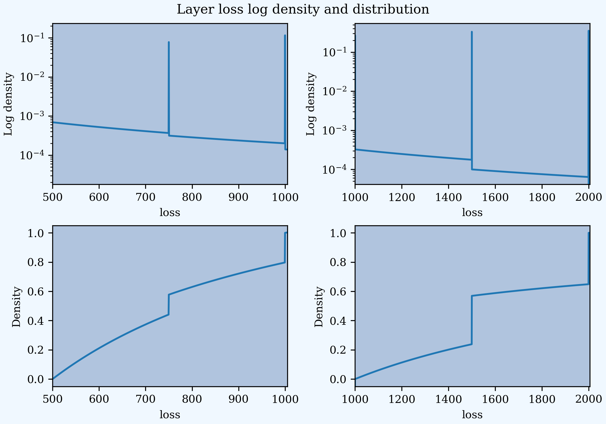
Mata et al. pay careful attention to the implied severity in each ceded layer, accounting for probability masses. They do this by considering losses in small intervals and weighting the underlying severity curves. aggregate automatically performs the same calculations to estimate the total layer severity. In this example, it uses a smaller bucket size of 0.5K compared to 2.5K in the original paper. The next plots reproduce [TODO Differences?!] Figures 2 and 3. The masses (spikes in density; jumps in distribution) occur when the lower limit unit has only limit losses.
In [191]: fig, axs = plt.subplots(2, 2, figsize=(2 * 3.5, 2 * 2.45), constrained_layout=True)

In [192]: ax0, ax1, ax2, ax3 = axs.flat

In [193]: (a19.density_df.p_sev / a19.sev.sf(500)).plot(xlim=[500, 1005],   logy=True, ax=ax0);

In [194]: (a19.density_df.p_sev / a19.sev.sf(1000)).plot(xlim=[1000, 2005], logy=True, ax=ax1);

In [195]: ((a19.density_df.F_sev - a19.sev.cdf(500)) / (a19.sev.cdf(1000) - a19.sev.cdf(500))).plot(xlim=[500, 1005], ylim=[-0.05, 1.05], ax=ax2);

In [196]: ((a19.density_df.F_sev - a19.sev.cdf(1000)) / (a19.sev.cdf(2000) - a19.sev.cdf(1000))).plot(xlim=[1000, 2005], ylim=[-0.05, 1.05], ax=ax3);

In [197]: for ax, y in zip(axs.flat, ['Log density', 'Log density', 'Density', 'Density']):
   .....:     ax.set(ylabel=y);
   .....:

In [198]: fig.suptitle('Layer loss log density and distribution');
Use an occurrence net of clause to apply the two excess of loss reinsurance layers. The estimated statistics refer to the net portfolio and reflect a pure exposure rating approach. Gross, ceded, and net expected losses are reported last.
In [199]: a19n = build('agg Re:MFV41n '
   .....:           '[1000 2000 2000 3000] premium at [.65 .65 .75 .75] lr '
   .....:           '[750 1000 1500 2000] xs [10 25 50 50] '
   .....:           'sev [exp(8)/1000 exp(8)/1000 exp(9)/1000 exp(9)/1000] * lognorm [2.5 2.5 3 3]  '
   .....:           'occurrence net of 500 xs 500 and 1000 xs 1000 '
   .....:           'poisson', bs=1/2)
   .....:

In [200]: qd(a19n)

       E[X] Est E[X] Err E[X]   CV(X) Est CV(X)  Skew(X) Est Skew(X)
X
Freq  22.51                   0.21077            0.21077
Sev  253.23   153.57 -0.39356  1.7344    1.1741   2.5007      1.0678
Agg    5700   3456.7 -0.39356 0.42198   0.32507  0.60601     0.39439
log2 = 16, bandwidth = 1/2, validation: n/a, reinsurance.

In [201]: print(f'Gross expected loss {a19.est_m:,.1f}\n'
   .....:       f'Ceded expected loss {a19.est_m - a19n.est_m:,.1f}\n'
   .....:       f'Net expected loss   {a19n.est_m:,.1f}')
   .....:
Gross expected loss 5,700.0
Ceded expected loss 2,243.3
Net expected loss   3,456.7
The reinsurance_audit_df dataframe summarizes ground-up (unconditional) layer loss statistics for occurrence covers. Thus, ex reports the layer severity per ground-up claim. The subject (gross) row is the same for all layers and replicates the gross severity statistics shown above for a.
In [202]: qd(a19n.reinsurance_audit_df.stack(0), sparsify=False)

                                     ex       var     sd     cv   skew
kind share limit  attach
occ  1.0   500.0  500.0  ceded   57.296     22247 149.15 2.6032  2.427
occ  1.0   500.0  500.0  net     195.93     93447 305.69 1.5602 2.5723
occ  1.0   500.0  500.0  subject 253.23 1.929e+05 439.21 1.7344 2.5007
occ  1.0   1000.0 1000.0 ceded   42.365     31584 177.72  4.195 4.4786
occ  1.0   1000.0 1000.0 net     210.86     94455 307.34 1.4575 1.6901
occ  1.0   1000.0 1000.0 subject 253.23 1.929e+05 439.21 1.7344 2.5007
occ  all   inf    gup    ceded    99.66     91341 302.23 3.0326 3.4354
occ  all   inf    gup    net     153.57     32509  180.3 1.1741 1.0678
occ  all   inf    gup    subject 253.23 1.929e+05 439.21 1.7344 2.5007
The reinsurance_occ_layer_df dataframe summarizes aggregate losses.
In [203]: qd(a19n.reinsurance_occ_layer_df, sparsify=False)

stat                    ex     ex      ex     cv     cv      cv     en severity     pct
view                 ceded    net subject  ceded    net subject  ceded    ceded   ceded
share limit  attach
1.0   500.0  500.0  1289.7 4410.3    5700 2.6032 1.5602  1.7344 3.5198   366.41 0.22626
1.0   1000.0 1000.0 953.61 4746.4    5700  4.195 1.4575  1.7344 1.5175   628.41  0.1673
all   inf    gup    2243.3 3456.7    5700 3.0326 1.1741  1.7344  22.51    99.66 0.39356
The layer severities show above differ slightly from Mata et al. Table 3. The aggregate computation is closest to Method 3. The reported severities are 351.1 and 628.8.
The reinsurance_df dataframe provides the gross, ceded, and net severity and aggregate distributions:
Severity distributions:
p_sev_gross,p_sev_ceded,p_sev_netAggregate distribution:
p_agg_gross_occ,p_agg_ceded_occ,p_agg_net_occshow the aggregate distributions computed using gross, cede, and net severity (occurrence) distributions. These are the portfolio gross, ceded and net distributions.The columns
p_agg_gross,p_agg_ceded,p_agg_netare relevant only when there is areoccurrenceandaggregatereinsurance clauses. They report gross, ceded and net of the aggregate covers, using the severity requested in the occurrence clause. In this casep_agg_grossis the same asp_agg_net_occbecause the occurrence clause specifiednet of.
Here is an extract from the severity distributions. Ceded severity is at most 1500. The masses at 250, 500, 1000 and 1500 are evident.
In [204]: qd(a19n.reinsurance_df.loc[0:2000:250,
   .....:     ['p_sev_gross', 'p_sev_ceded', 'p_sev_net']])
   .....:

        p_sev_gross  p_sev_ceded  p_sev_net
loss
0.0       0.0059219      0.84369  0.0059219
125.0    0.00074474   7.6472e-05 0.00074474
250.0    0.00029874     0.012139 0.00029874
375.0    0.00016663   3.8634e-05 0.00016663
500.0    0.00010806     0.018065    0.15642
625.0    7.6472e-05   1.8367e-05          0
750.0      0.012139   1.5689e-05          0
875.0    3.8634e-05   1.3584e-05          0
1000.0     0.018065     0.022295          0
1125.0   1.8367e-05   5.9515e-06          0
1250.0   1.5689e-05   5.3056e-06          0
1375.0   1.3584e-05   4.7639e-06          0
1500.0     0.022295     0.023679          0
1625.0   5.9515e-06            0          0
1750.0   5.3056e-06            0          0
1875.0   4.7639e-06            0          0
2000.0     0.023679            0          0
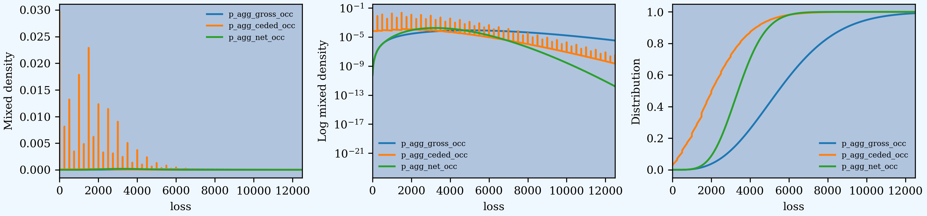
Here is an extract from the aggregate distributions, followed by the density and distribution plots. The masses are caused by outcomes involving only limit losses.
In [205]: qd(a19n.reinsurance_df.loc[3000:6000:500,
   .....:     ['p_agg_gross_occ', 'p_agg_ceded_occ', 'p_agg_net_occ']])
   .....:

        p_agg_gross_occ  p_agg_ceded_occ  p_agg_net_occ
loss
3000.0       5.6326e-05        0.0090335     0.00017503
3250.0       6.2846e-05        0.0024374     0.00017886
3500.0       6.8727e-05        0.0050447     0.00017401
3750.0       7.3779e-05        0.0013535     0.00016174
4000.0       7.7914e-05        0.0037091     0.00014418
4250.0       8.1081e-05        0.0010054     0.00012359
4500.0        8.328e-05         0.002359     0.00010216
4750.0       8.4511e-05       0.00063735     8.1596e-05
5000.0       8.4787e-05        0.0012892     6.3111e-05
5250.0       8.4135e-05       0.00034824      4.735e-05
5500.0       8.2634e-05       0.00080992     3.4517e-05
5750.0       8.0373e-05       0.00022017     2.4482e-05
6000.0       7.7463e-05       0.00045425     1.6918e-05

In [206]: fig, axs = plt.subplots(1, 3, figsize=(3 * 3.5, 2.45), constrained_layout=True)

In [207]: ax0, ax1, ax2 = axs.flat

In [208]: bit = a19n.reinsurance_df[['p_agg_gross_occ', 'p_agg_ceded_occ', 'p_agg_net_occ']]

In [209]: bit.plot(ax=ax0);

In [210]: bit.plot(logy=True, ax=ax1);

In [211]: bit.cumsum().plot(ax=ax2);

In [212]: for ax in axs.flat:
   .....:     ax.set(xlim=[0, 12500]);
   .....:

In [213]: ax0.set(ylabel='Mixed density');

In [214]: ax1.set(ylabel='Log mixed density');

In [215]: ax2.set(ylabel='Distribution');
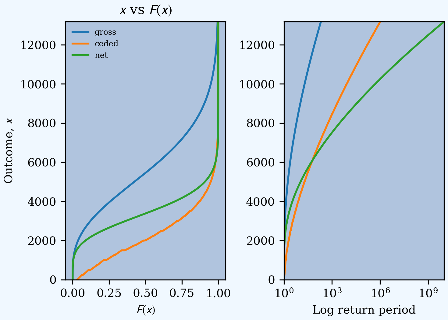
Any desired risk management evaluation can be computed from reinsurance_df, which contains the gross, ceded, and net distributions. For example, here is a tail return period plot and a dataframe of summary statistics.
In [216]: fig, axs = plt.subplots(1, 2, figsize=(2 * 2.45, 3.5), constrained_layout=True)

In [217]: ax0, ax1 = axs.flat

In [218]: for c in bit.columns:
   .....:     ax0.plot(bit[c].cumsum(), bit.index, label=c.split('_')[2])
   .....:     rp = 1 / (1 - bit[c].cumsum())
   .....:     ax1.plot(rp, bit.index, label=c)
   .....:

In [219]: ax0.xaxis.set_major_locator(ticker.MultipleLocator(0.25))

In [220]: ax0.set(ylim=[0, a19n.q(1-1e-10)], title='$x$ vs $F(x)$', xlabel='$F(x)$', ylabel='Outcome, $x$');

In [221]: ax1.set(xscale='log', xlim=[1, 1e10], ylim=[0, a19n.q(1-1e-10)], xlabel='Log return period');

In [222]: ax0.legend(loc='upper left');

In [223]: df = pd.DataFrame({c.split('_')[2]: xsden_to_meancvskew(bit.index, bit[c]) for c in bit.columns},
   .....:              index=['mean', 'cv', 'skew'])
   .....:

In [224]: qd(df)

       gross   ceded     net
mean    5700  2243.3  3456.7
cv   0.42198 0.67304 0.32507
skew 0.60601  0.8053 0.39439
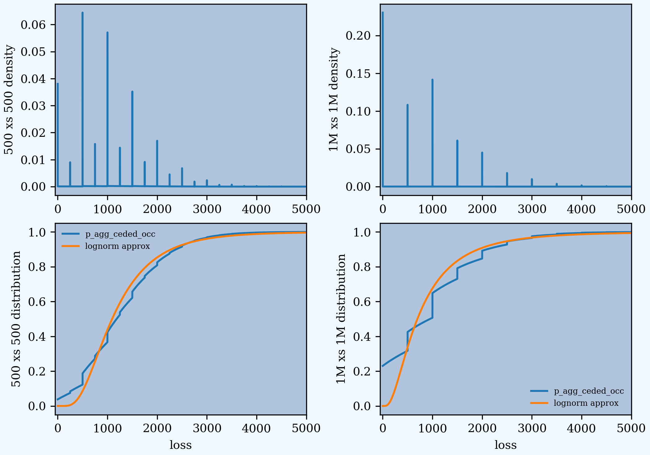
Mata Figures 4, 5, 6 and 7 show the aggregate mixed density and distribution functions for each layer. These plots are replicated below. Our model uses a gamma mixed Poisson frequency with a variance multiplier of 2.0, resulting in a lower variance multiplier for excess layers (see REF). The plots in Mata appear to use a variance multiplier of 2.0 for the excess layer, resulting in a more skewed distribution.
In [225]: from aggregate import lognorm_approx

In [226]: vm = 2.0; c = (vm - 1) / a19.n; cv = c**0.5

In [227]: a20 = build('agg Re:MFV41n1 '
   .....:           '[1000 2000 2000 3000] premium at [.65 .65 .75 .75] lr '
   .....:           '[750 1000 1500 2000] xs [10 25 50 50] '
   .....:           'sev [exp(8)/1000 exp(8)/1000 exp(9)/1000 exp(9)/1000] * lognorm [2.5 2.5 3 3]  '
   .....:           'occurrence net of 500 xs 500 '
   .....:           f'mixed gamma {cv}', bs=1/2)
   .....:

In [228]: a21 = build('agg Re:MFV41n2 '
   .....:           '[1000 2000 2000 3000] premium at [.65 .65 .75 .75] lr '
   .....:           '[750 1000 1500 2000] xs [10 25 50 50] '
   .....:           'sev [exp(8)/1000 exp(8)/1000 exp(9)/1000 exp(9)/1000] * lognorm [2.5 2.5 3 3]  '
   .....:           'occurrence net of 1000 xs 1000 '
   .....:           f'mixed gamma {cv}', bs=1/2)
   .....:

In [229]: qd(a20)

       E[X] Est E[X] Err E[X]   CV(X) Est CV(X)  Skew(X) Est Skew(X)
X
Freq  22.51                   0.29808            0.44712
Sev  253.23   195.93 -0.22626  1.7344    1.5602   2.5007      2.5723
Agg    5700   4410.3 -0.22626  0.4717   0.44384  0.69763     0.68565
log2 = 16, bandwidth = 1/2, validation: n/a, reinsurance.

In [230]: qd(a21)

       E[X] Est E[X] Err E[X]   CV(X) Est CV(X)  Skew(X) Est Skew(X)
X
Freq  22.51                   0.29808            0.44712
Sev  253.23   210.86  -0.1673  1.7344    1.4575   2.5007      1.6901
Agg    5700   4746.4  -0.1673  0.4717   0.42805  0.69763     0.60342
log2 = 16, bandwidth = 1/2, validation: n/a, reinsurance.

In [231]: fig, axs = plt.subplots(2, 2, figsize=(2 * 3.5, 2 * 2.45), constrained_layout=True); \
   .....: ax0, ax1, ax2, ax3 = axs.flat; \
   .....: a20.reinsurance_df.p_agg_ceded_occ.plot(ax=ax0); \
   .....: a20.reinsurance_df.p_agg_ceded_occ.cumsum().plot(ax=ax2); \
   .....: a21.reinsurance_df.p_agg_ceded_occ.plot(ax=ax1); \
   .....: a21.reinsurance_df.p_agg_ceded_occ.cumsum().plot(ax=ax3); \
   .....: xs = np.linspace(0, 5000, 501); \
   .....: fz = lognorm_approx(a20.reinsurance_df.p_agg_ceded_occ); \
   .....: ax2.plot(xs, fz.cdf(xs), label='lognorm approx'); \
   .....: fz = lognorm_approx(a21.reinsurance_df.p_agg_ceded_occ); \
   .....: ax3.plot(xs, fz.cdf(xs), label='lognorm approx'); \
   .....: ax2.legend(); \
   .....: ax3.legend(); \
   .....: ax0.set(xlim=[-50, 5000], xlabel=None, ylabel='500 xs 500 density'); \
   .....: ax2.set(xlim=[-50, 5000], ylabel='500 xs 500 distribution'); \
   .....: ax1.set(xlim=[-50, 5000], xlabel=None, ylabel='1M xs 1M density');
   .....:

In [232]: ax3.set(xlim=[-50, 5000], ylabel='1M xs 1M distribution');
2.6.10. Summary of Objects Created by DecL
Objects created by build() in this guide.
In [233]: from aggregate import pprint_ex

In [234]: for n, r in build.qlist('^(Re):').iterrows():
   .....:     pprint_ex(r.program, split=20)
   .....:
agg Re:01
  dfreq [1 2 3 4 5 6]
  dsev [1 2 3 4 5 6]
agg Re:02
  dfreq [1:6]
  dsev [1:6]
  occurrence net of 1 xs 4 and 1 xs 5
agg Re:03
  agg.Re:01
  aggregate ceded to 6 xs 24 and 6 xs 30
agg Re:04
  dfreq [1:6]
  dsev [1:6]
  occurrence net of 1 xs 4 and 1 xs 5
  aggregate net of 4 xs 12 and 4 xs 16
agg Re:05
  dfreq [1:6]
  dsev [1:6]
  occurrence net of 0.5 so 2 xs 2 and 2 xs 4
  aggregate net of 1 po 4 xs 10
agg Re:06
  agg.Re:01
  aggregate ceded to tower [0 1 2 5 10 20 36]
agg Re:07 [10000 5000 2500 1500] premium at [0.75 0.75 0.7 0.65] lr [ 1000 2000 5000 10000] xs [ 0 0 100 250]
  sev lognorm 50 cv 10
  occurrence ceded to tower [0 250 500 1000 2000 5000 10000]
  poisson
agg Re:08 [ 2.975 3.325 4.375 5.25 15.75 28. 31.5 42. 87.5 175. ] premium at [0.55 0.55 0.55 0.55 0.55 0.55 0.55 0.55 0.55 0.55] lr [ 850 950 1250 1500 4500 8000 9000 12000 25000 50000] xs [ 10 10 20 20 50 100 500 1000 5000 5000]
  sev [ 850 950 1250 1500 4500 8000 9000 12000 25000 50000] * beta 0.4253774182673055 1.093686593600036 !
  occurrence ceded to tower [0 1000 5000 10000 20000 inf]
  mixed gamma 2
agg Re:09 [ 2.975 3.325 4.375 5.25 15.75 28. 31.5 42. 87.5 175. ] premium at [0.55 0.55 0.55 0.55 0.55 0.55 0.55 0.55 0.55 0.55] lr [ 850 950 1250 1500 4500 8000 9000 12000 25000 50000] xs [ 10 10 20 20 50 100 500 1000 5000 5000]
  sev [ 850 950 1250 1500 4500 8000 9000 12000 25000 50000] * beta 0.4253774182673055 1.093686593600036 !
  occurrence ceded to 4000 xs 1000 and 5000 xs 5000
  mixed gamma 2
agg Re:BN1 [9000 3000] exposure at [0.04 0.03] rate 160 xs 0
  sev 40 * pareto [0.9 0.95] - 40
  mixed gamma 0.08357551150546018
agg Re:BN1a [9000 3000] exposure at [0.04 0.03] rate 160 xs 0
  sev 40 * pareto [0.9 0.95] - 40
  mixed gamma 0.08357551150546018
  aggregate net of 360 xs 0
agg Re:BN1c [9000 3000] exposure at [0.04 0.03] rate 160 xs 0
  sev 40 * pareto [0.9 0.95] - 40
  mixed gamma 0.05**.5
  aggregate net of 360 xs 0
agg Re:BN1p [9000 3000] exposure at [0.04 0.03] rate 160 xs 0
  sev 40 * pareto [0.9 0.95] - 40
  poisson
  aggregate net of 360 xs 0
agg Re:BN2 [2000 2000 2000] exposure at [.1 .14 .21] rate 700 xs 0
  sev 300 * pareto [1.5 1.3 1.1] - 300
  mixed gamma 0.07
agg Re:BN2a [2000 2000 2000] exposure at [.1 .14 .21] rate 700 xs 0
  sev 300 * pareto [1.5 1.3 1.1] - 300
  mixed gamma 0.07
  aggregate ceded to 2800 xs 0
agg Re:BN2p [2000 2000 2000] exposure at [.1 .14 .21] rate 700 xs 0
  sev 300 * pareto [1.5 1.3 1.1] - 300
  poisson
agg Re:BN3 [4500 4500 1000] exposure at [.032 .038 .035] rate 400 xs 0
  sev 100 * pareto 1.1 - 100
  poisson
agg Re:BN3lc [4500 4500 1000] exposure at [.032 .038 .035] rate 400 xs 0
  sev 100 * pareto 1.1 - 100
  poisson
  aggregate net of 350 xs 350
agg Re:BN4 [9000 3000] exposure at [0.04 0.03] rate 160 xs 0
  sev 40 * pareto [0.9 0.95] - 40
  poisson
agg Re:BN5
  25000 exposure at 0.1 rate 900 xs 0
  sev 100 * pareto 1.05 - 100
  mixed gamma 0.095
agg Re:BN6c [6000 6000 6000] exposure at [.1 .14 .21] rate 700 xs 0
  sev 300 * pareto [1.5 1.3 1.1] - 300
  mixed gamma 0.1**.5
agg Re:BN6p [6000 6000 6000] exposure at [.1 .14 .21] rate 700 xs 0
  sev 300 * pareto [1.5 1.3 1.1] - 300
  poisson
agg Re:MFV41 [1000 2000 2000 3000] premium at [.65 .65 .75 .75] lr [750 1000 1500 2000] xs [10 25 50 50]
  sev [exp(8)/1000 exp(8)/1000 exp(9)/1000 exp(9)/1000] * lognorm [2.5 2.5 3 3]
  poisson
agg Re:MFV41n [1000 2000 2000 3000] premium at [.65 .65 .75 .75] lr [750 1000 1500 2000] xs [10 25 50 50]
  sev [exp(8)/1000 exp(8)/1000 exp(9)/1000 exp(9)/1000] * lognorm [2.5 2.5 3 3]
  occurrence net of 500 xs 500 and 1000 xs 1000
  poisson
agg Re:MFV41n1 [1000 2000 2000 3000] premium at [.65 .65 .75 .75] lr [750 1000 1500 2000] xs [10 25 50 50]
  sev [exp(8)/1000 exp(8)/1000 exp(9)/1000 exp(9)/1000] * lognorm [2.5 2.5 3 3]
  occurrence net of 500 xs 500
  mixed gamma 0.21077377162538105
agg Re:MFV41n2 [1000 2000 2000 3000] premium at [.65 .65 .75 .75] lr [750 1000 1500 2000] xs [10 25 50 50]
  sev [exp(8)/1000 exp(8)/1000 exp(9)/1000 exp(9)/1000] * lognorm [2.5 2.5 3 3]
  occurrence net of 1000 xs 1000
  mixed gamma 0.21077377162538105