2.1. Student
Objectives: Introduction to aggregate distributions using simple discrete examples for actuarial science majors and short-term actuarial modeling exam candidates; get started using aggregate.
Audience: New user, with no knowledge of aggregate distributions or insurance terminology.
Prerequisites: Basic probability theory; Python and pandas programming.
See also: Actuarial Student.
Contents:
Formal Construction
Simple Example
Exercise - Test Your Understanding
Dice Rolls
2.1.1. What Is an Aggregate Probability Distribution?
An aggregate probability distribution describes the sum of a random number of identically distributed outcome random variables. The distribution of the number called the frequency distribution and of the outcome the severity distribution.
Examples.
Total losses from insurance claims from a portfolio of policies: frequency equals the number of claims and the severity outcome is the amount of each claim.
Larvae per unit area (Neyman 1939): frequency is the number of egg clusters per unit area and severity is the number of larvae per egg cluster.
Number of vehicle occupants passing a point on the road: frequency is the number of vehicles passing the point and severity is the number of occupants per vehicle.
Total transaction value in an exchange: frequency is the number of transactions and severity is the amount of each transaction.
Aggregate distributions are used in many fields and go by different names, including compound distributions, generalized distributions, and stopped-sum distributions.
2.1.2. Formal Construction
Let \(N\) be a discrete random variable taking non-negative integer values. Its outcomes give the frequency (number) of events. Let \(X_i\) be a series of independent, identically distributed (iid) severity random variables modeling an outcome. An aggregate distribution is the distribution of the random sum
\(N\) is called the frequency component of the aggregate and \(X\) the severity.
An observation from \(A\) is realized by:
Sample (or simulate) an outcome \(n\) from \(N\)
For \(i=1,\dots, n\), sample \(X_i\)
Return \(A:=X_1 + \cdots + X_n\)
It is usual to assume that \(X\) and \(N\) are independent. Check this assumption is reasonable for your use case; it is not always appropriate. For example, consider modeling hourly takings from a shop checkout till as the number of customers served (frequency) and the amount spent by each customer (severity). Larger orders take longer to tabulate and so frequency is negatively correlated with severity. Example 4 above assumes large orders on an exchange are transacted as quickly as small ones.
2.1.3. Simple Example
Frequency \(N\) can equal 1, 2, or 3, with probabilities 1/2, 1/4, and 1/4.
Severity \(X\) can equal 1, 2, or 4, with probabilities 5/8, 1/4, and 1/8.
Aggregate \(A = X_1 + \cdots + X_N\).
Exercise.
What are the expected value and CV of \(N\)?
What are the expected value and CV of \(X\)?
What are the expected value and CV of \(A\)?
What possible values can \(A\) take? What are the probabilities of each?
Important
Stop and solve the exercise!
The exercise is not difficult, but it requires careful bookkeeping and attention to detail. It would soon become impractical to solve by hand if there were more outcomes for frequency or severity. This is where aggregate comes in. It can solve exercise in the following few lines of code, which we now go through step-by-step.
The first line imports build and a helper “quick display” function qd. You almost always want to start this way.
In [1]: from aggregate import build, qd
The next three lines specify the aggregate using a Dec Language (DecL) program to describe its frequency and severity components.
In [2]: a01 = build('agg Student:01 '
   ...:             'dfreq [1 2 3] [1/2 1/4 1/4] '
   ...:             'dsev [1 2 4] [5/8 1/4 1/8]')
   ...:
The DecL program has three parts:
aggis a keyword andStudent:01is a user-selected name. Names must start with a letter and can include numbers and colons. This clause declares that we are building an aggregate distribution.dfreqis a keyword to specify the frequency distribution. The next two blocks of numbers are the outcomes[1 2 3]and their probabilities[1/2 1/4 1/4]. Commas are optional in the lists and only division arithmetic is supported.dsevis a keyword to specify the a discrete severity distribution. It has the same outcomes-probabilities form asdfreq.
The program string is only one line long because Python automatically concatenates strings within parenthesis; it is split up for clarity. It is recommended that DecL programs be split in this way. Note the spaces at the end of each line, see 10 mins formatting.
Use qd to print a dataframe of statistics that answer the first three questions: the mean and CV for the frequency (Freq), severity (Sev) and aggregate (Agg) distributions.
In [3]: qd(a01)

       E[X] Est E[X]    Err E[X]   CV(X) Est CV(X)  Skew(X) Est Skew(X)
X
Freq   1.75                       0.4738            0.49338
Sev   1.625    1.625           0 0.61056   0.61056   1.5719      1.5719
Agg  2.8438   2.8437 -1.1102e-16 0.66144   0.66144   1.0808      1.0808
log2 = 5, bandwidth = 1, validation: not unreasonable.
The columns E[X], CV(X), and Skew(X) report the mean, CV, and skewness for each component computed analytically or very accurately with numerical integration.
The columns Est E[X], Est CV(X), and Est Skew(X) are computed numerically by aggregate. For discrete models they equal the analytic answer because the only errors introduced by aggregate come from discretizing the severity distribution. That is also why there are no estimates for frequency. Err E[X] shows the error (difference, not relative error) in the mean. This handy dataframe can be accessed directly via the property a01.describe. The note log2 = 5, bs = 1 describe the inner workings, discussed in REF.
It remains to give the aggregate probability mass function. It is available in the dataframe a01.density_df. Here are the probability masses, and distribution and survival functions evaluated for all possible aggregate outcomes.
In [4]: qd(a01.density_df.query('p_total > 0')[['p_total', 'F', 'S']])

        p_total       F          S
loss
1.0      0.3125  0.3125     0.6875
2.0     0.22266 0.53516    0.46484
3.0     0.13916 0.67432    0.32568
4.0     0.15137 0.82568    0.17432
5.0    0.068359 0.89404    0.10596
6.0    0.056152  0.9502   0.049805
7.0    0.029297 0.97949   0.020508
8.0   0.0097656 0.98926   0.010742
9.0   0.0073242 0.99658   0.003418
10.0  0.0029297 0.99951 0.00048828
12.0 0.00048828       1          0
The possible outcomes range from 1 (frequency 1, outcome 1) to 12 (frequency 3, all outcomes 4). It is easy to check the reported probabilities are correct. It is impossible to obtain an outcome of 11.
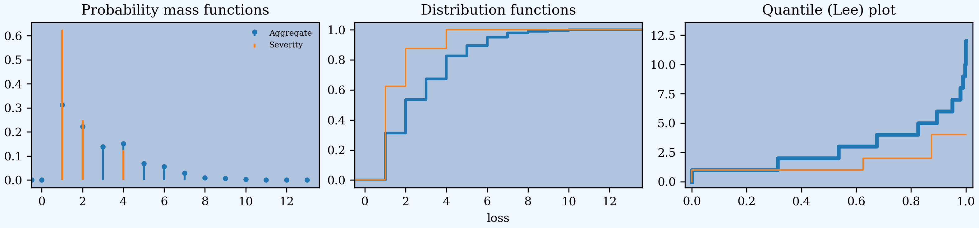
For extra credit, here is a plot of the pmf, cdf, and the outcome Lee diagram, showing the severity and aggregate. These are produced automatically by a01.plot() from the density_df dataframe.
In [5]: a01.plot()
2.1.4. Exercise - Test Your Understanding
Frequency: 1, 2 or 3 events; 50% chance of 1 event, 25% chance of 2, and 25% chance of 3.
Severity: 1, 2, 4, 8 or 16, each with equal probability.
What is the average frequency?
What is the average severity?
What are the average aggregate?
What is the aggregate coefficient of variation?
Tabulate the probability of all possible aggregate outcomes.
First, try by hand and then using aggregate.
Here is the aggregate solution. The probability clause in dsev can be omitted when all outcomes are equally likely. The moments and CVs are shown in the table.
In [6]: a02 = build('agg Student:02 '
   ...:             'dfreq [1 2 3] [.5 .25 .25] '
   ...:             'dsev [1 2 4 8 16] ')
   ...:

In [7]: qd(a02)

      E[X] Est E[X]    Err E[X]   CV(X) Est CV(X)  Skew(X) Est Skew(X)
X
Freq  1.75                       0.4738            0.49338
Sev    6.2      6.2 -1.1102e-16 0.87988   0.87988  0.88905     0.88905
Agg  10.85    10.85 -1.1102e-16 0.81663   0.81663   1.0066      1.0066
log2 = 7, bandwidth = 1, validation: not unreasonable.
All possible aggregate outcomes are shown next. The largest outcome of 48 has probability 1/4 * (1/5)**3 = 1/500 = 0.002.
In [8]: qd(a02.density_df.query('p_total > 0')[['p_total', 'F', 'S']])

      p_total     F           S
loss
1.0       0.1   0.1         0.9
2.0      0.11  0.21        0.79
3.0     0.022 0.232       0.768
4.0     0.116 0.348       0.652
5.0     0.026 0.374       0.626
6.0     0.028 0.402       0.598
7.0     0.012 0.414       0.586
8.0     0.116  0.53        0.47
9.0     0.026 0.556       0.444
10.0    0.032 0.588       0.412
11.0    0.012   0.6         0.4
12.0    0.028 0.628       0.372
...       ...   ...         ...
21.0    0.012 0.882       0.118
22.0    0.012 0.894       0.106
24.0    0.028 0.922       0.078
25.0    0.012 0.934       0.066
26.0    0.012 0.946       0.054
28.0    0.012 0.958       0.042
32.0    0.016 0.974       0.026
33.0    0.006  0.98        0.02
34.0    0.006 0.986       0.014
36.0    0.006 0.992       0.008
40.0    0.006 0.998       0.002
48.0    0.002     1 -2.2204e-16

In [9]: a02.plot()

2.1.5. Dice Rolls
This section presents a series of examples involving dice rolls. The early examples are useful because you know the answer and can see aggregate is correct.
2.1.5.1. One Dice Roll
The DecL program for one dice roll.
In [10]: one_dice = build('agg Student:01Dice '
   ....:                  'dfreq [1] '
   ....:                  'dsev [1:6]')
   ....:

In [11]: one_dice.plot()

In [12]: qd(one_dice)

      E[X] Est E[X] Err E[X]   CV(X) Est CV(X) Skew(X) Est Skew(X)
X
Freq     1                         0
Sev    3.5      3.5        0 0.48795   0.48795       0  2.8529e-15
Agg    3.5      3.5        0 0.48795   0.48795       0  8.5588e-15
log2 = 4, bandwidth = 1, validation: not unreasonable.

2.1.5.2. Two Dice Rolls
The program for two dice rolls produces a triangular aggregate distribution, as shown in the table and illustrated in the graph (left, probability mass function in blue).
In [13]: import numpy as np

In [14]: two_dice = build('agg Student:02Dice '
   ....:                  'dfreq [2] '
   ....:                  'dsev [1:6]')
   ....:

In [15]: two_dice.plot()

In [16]: qd(two_dice)

      E[X] Est E[X]    Err E[X]   CV(X) Est CV(X) Skew(X) Est Skew(X)
X
Freq     2                            0
Sev    3.5      3.5           0 0.48795   0.48795       0  2.8529e-15
Agg      7        7 -3.3307e-16 0.34503   0.34503       0 -4.0346e-14
log2 = 5, bandwidth = 1, validation: not unreasonable.

In [17]: bit = two_dice.density_df.query('p_total > 0')[['p_total', 'F', 'S']]

In [18]: bit['36p'] = np.round(bit.p_total * 36)

In [19]: bit['36p'] = bit['36p'].astype(int)

In [20]: qd(bit)

      p_total        F           S  36p
loss
2.0  0.027778 0.027778     0.97222    1
3.0  0.055556 0.083333     0.91667    2
4.0  0.083333  0.16667     0.83333    3
5.0   0.11111  0.27778     0.72222    4
6.0   0.13889  0.41667     0.58333    5
7.0   0.16667  0.58333     0.41667    6
8.0   0.13889  0.72222     0.27778    5
9.0   0.11111  0.83333     0.16667    4
10.0 0.083333  0.91667    0.083333    3
11.0 0.055556  0.97222    0.027778    2
12.0 0.027778        1 -2.2204e-16    1

2.1.5.3. Twelve Dice Rolls
The aggregate program for twelve dice rolls, which is much harder to compute by hand!
In [21]: twelve_dice = build('agg Student:12Dice '
....: 'dfreq [12] '
....: 'dsev [1:6]')
....:
In [22]: qd(twelve_dice)
E[X] Est E[X] Err E[X] CV(X) Est CV(X) Skew(X) Est Skew(X)
X
Freq 12 0
Sev 3.5 3.5 0 0.48795 0.48795 0 2.8529e-15
Agg 42 42 1.9984e-15 0.14086 0.14086 0 1.4337e-11
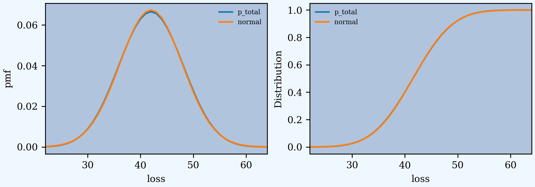
log2 = 8, bandwidth = 1, validation: not unreasonable.
The distribution compared to a moment-matched normal approximation. fz is a scipy.stats normal random variable created using the approximate method. The last two plots show very good convergence to the central limit theorem normal distribution.
In [23]: import matplotlib.pyplot as plt

In [24]: fz = twelve_dice.approximate('norm')

In [25]: df = twelve_dice.density_df[['p_total', 'F', 'S']]

In [26]: df['normal'] = np.diff(fz.cdf(df.index + 0.5), prepend=0)

In [27]: qd(df.iloc[32:52])

      p_total        F        S   normal
loss
32.0 0.016609 0.054298   0.9457 0.016196
33.0 0.021737 0.076034  0.92397 0.021233
34.0 0.027592  0.10363  0.89637 0.027054
35.0 0.033997  0.13762  0.86238 0.033502
36.0  0.04069  0.17831  0.82169 0.040322
37.0  0.04733  0.22564  0.77436 0.047165
38.0  0.05353  0.27917  0.72083  0.05362
39.0 0.058887  0.33806  0.66194 0.059245
40.0 0.063026  0.40109  0.59891 0.063621
41.0 0.065643  0.46673  0.53327   0.0664
42.0 0.066539  0.53327  0.46673 0.067353
43.0 0.065643  0.59891  0.40109   0.0664
44.0 0.063026  0.66194  0.33806 0.063621
45.0 0.058887  0.72083  0.27917 0.059245
46.0  0.05353  0.77436  0.22564  0.05362
47.0  0.04733  0.82169  0.17831 0.047165
48.0  0.04069  0.86238  0.13762 0.040322
49.0 0.033997  0.89637  0.10363 0.033502
50.0 0.027592  0.92397 0.076034 0.027054
51.0 0.021737   0.9457 0.054298 0.021233

In [28]: fig, axs = plt.subplots(1, 2, figsize=(2 * 3.5, 2.45), constrained_layout=True); \
   ....: ax0, ax1 = axs.flat; \
   ....: df[['p_total', 'normal']].plot(xlim=[22, 64], ax=ax0); \
   ....: ax0.set(ylabel='pmf'); \
   ....: df[['p_total', 'normal']].cumsum().plot(xlim=[22, 64], ax=ax1);
   ....:

In [29]: ax1.set(ylabel='Distribution');
2.1.5.4. A Dice Roll of Dice Rolls
The last example is a dice roll of dice rolls: throw a dice, then throw that many dice and add up the dots. The result range from 1 (throw 1 first, then 1 again) to 36 (throw 6 first, then 6 for each of the six die).
In [30]: dd = build('agg Student:DD '
   ....:            'dfreq [1:6] '
   ....:            'dsev [1:6]')
   ....:

In [31]: qd(dd)

      E[X] Est E[X]   Err E[X]   CV(X) Est CV(X)  Skew(X) Est Skew(X)
X
Freq   3.5                     0.48795                  0
Sev    3.5      3.5          0 0.48795   0.48795        0  2.8529e-15
Agg  12.25    12.25 1.5543e-15 0.55328   0.55328  0.28689     0.28689
log2 = 7, bandwidth = 1, validation: not unreasonable.

In [32]: dd.plot()
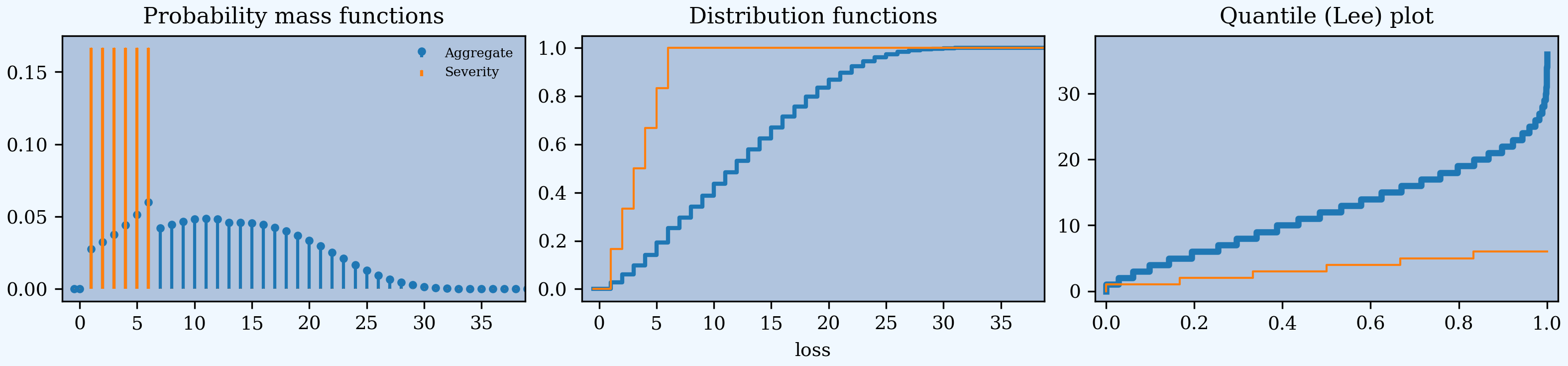
The largest outcome of 36 has probability 6**-7. See below for a check of the accuracy. Work out the probability of 6 or 7 to better appreciate the work performed by aggregate! Why is there a sudden drop between 6 and 7 in the (blue) probability mass function (left hand plot)?
In [33]: import pandas as pd

In [34]: a, e = (1/6)**7, dd.density_df.loc[36, 'p_total']

In [35]: pd.DataFrame([a, e, e/a-1],
   ....:     index=['Actual worst', 'Computed worst', 'error'],
   ....:     columns=['value'])
   ....:
Out[35]:
                       value
Actual worst    3.572245e-06
Computed worst  3.572245e-06
error           1.178835e-12
We return to this example in Reinsurance Pricing.
2.1.6. Summary of Objects Created by DecL
Objects created by build() in this guide.
In [36]: from aggregate import pprint_ex

In [37]: for n, r in build.qlist('^Student:').iterrows():
   ....:     pprint_ex(r.program, split=20)
   ....:
agg Student:01
  dfreq [1 2 3] [1/2 1/4 1/4]
  dsev [1 2 4] [5/8 1/4 1/8]
agg Student:01Dice
  dfreq [1]
  dsev [1:6]
agg Student:02
  dfreq [1 2 3] [.5 .25 .25]
  dsev [1 2 4 8 16]
agg Student:02Dice
  dfreq [2]
  dsev [1:6]
agg Student:12Dice
  dfreq [12]
  dsev [1:6]
agg Student:DD
  dfreq [1:6]
  dsev [1:6]