2.12. Working With Samples
Objectives: How to sample from aggregate and how to a build a Portfolio from a sample. Inducing correlation in a sample using the Iman-Conover algorithm and determining the worst-VaR rearrangement using the rearrangement algorithm.
Audience: Planning and strategy, ERM, capital modeling, risk management actuaries.
Prerequisites: DecL, aggregate distributions, risk measures.
See also: Using Samples and The Switcheroo Trick, The Iman-Conover Method, The Rearrangement Algorithm.
Contents:
Helpful References
2.12.1. Helpful References
2.12.2. Samples and Densities
Use case: make realistic marginal distributions with aggregate that reflect the underlying frequency and severity (rather than defaulting to a lognormal determined by a CV assumption) and then use a sample in your simulation model.
2.12.3. Samples from aggregate Object
The method sample() draws a sample from an Aggregate or Portfolio
class object. Both cases work by applying pandas.DataFrame.sample to the object’s density_df dataframe.
Examples.
A sample from an
Aggregate. Set up a simple lognormal distribution, modeled as an aggregate with trivial frequency.
In [1]: from aggregate import build, qd, set_seed

In [2]: a01 = build('agg Samp:01 '
   ...:           '1 claim '
   ...:           'sev lognorm 10 cv .4 '
   ...:           'fixed'
   ...:          , bs=1/512)
   ...:

In [3]: qd(a01)

      E[X] Est E[X]    Err E[X]  CV(X) Est CV(X) Skew(X) Est Skew(X)
X
Freq     1                           0
Sev     10       10 -6.1087e-11    0.4       0.4   1.264       1.264
Agg     10       10 -6.1087e-11    0.4       0.4   1.264       1.264
log2 = 16, bandwidth = 1/512, validation: not unreasonable.
Apply
sample()and display the results.In [4]: set_seed(102) In [5]: df = a01.sample(10**5) In [6]: fc = lambda x: f'{x:8.2f}' In [7]: qd(df.head(), float_format=fc) loss 0 6.33 1 10.10 2 13.29 3 7.56 4 11.18The sample histogram and the computed pmf are close. The pmf is adjusted to the resolution of the histogram.
In [8]: fig, ax = plt.subplots(1, 1, figsize=(3.5, 2.45), constrained_layout=True)

In [9]: xm = a01.q(0.999)

In [10]: df.hist(bins=np.arange(xm), ec='w', lw=.25, density=True,
   ....:     ax=ax, grid=False);
   ....:

In [11]: (a01.density_df.loc[:xm, 'p_total'] / a01.bs).plot(ax=ax);

In [12]: ax.set(title='Sample and aggregate pmf', ylabel='pmf');
A sample from a
Portfolioproduces a multivariate distribution. Setup a simplePortfoliowith three lognormal marginals.
In [13]: from aggregate.utilities import qdp

In [14]: from pandas.plotting import scatter_matrix

In [15]: p02 = build('port Samp:02 '
   ....:         'agg A 1 claim sev lognorm 10 cv .2 fixed '
   ....:         'agg B 1 claim sev lognorm 15 cv .5 fixed '
   ....:         'agg C 1 claim sev lognorm  5 cv .8 fixed '
   ....:        , bs=1/128)
   ....:

In [16]: qd(p02)

            E[X] Est E[X]    Err E[X]   CV(X) Est CV(X) Skew(X) Est Skew(X)
unit  X
A     Freq     1                            0
      Sev     10       10 -2.2204e-16     0.2       0.2   0.608       0.608
      Agg     10       10 -2.2204e-16     0.2       0.2   0.608       0.608
B     Freq     1                            0
      Sev     15       15 -2.2282e-13     0.5       0.5   1.625       1.625
      Agg     15       15 -2.2282e-13     0.5       0.5   1.625       1.625
C     Freq     1                            0
      Sev      5        5 -2.3183e-10     0.8       0.8   2.912       2.912
      Agg      5        5 -2.3183e-10     0.8       0.8   2.912       2.912
total Freq     3                            0
      Sev     10       10  -3.875e-11 0.64872            1.8077
      Agg     30       30 -6.3166e-11 0.29107   0.29107  1.3168      1.3168
log2 = 16, bandwidth = 1/128, validation: not unreasonable.
Apply
sample()to produce a sample with no correlation. Here are the first few values.In [17]: df = p02.sample(10**4) In [18]: qd(df.head(), float_format=fc) A B C total 0 9.45 21.07 4.86 35.38 1 11.73 20.10 8.34 40.16 2 10.93 12.06 3.05 26.05 3 7.24 6.34 1.79 15.37 4 8.28 13.30 13.87 35.45
qdp()prints the pandasdescribestatistics dataframe for a dataframe, and adds the CV.In [19]: qdp(df) Out[19]: A B C total count 10000.000000 10000.000000 10000.000000 10000.000000 mean 9.966709 15.052769 5.058216 30.077694 std 2.002445 7.583697 4.047945 8.889127 min 3.664062 2.117188 0.250000 11.726562 25% 8.539062 9.773438 2.484375 23.781250 50% 9.789062 13.351562 4.000000 28.507812 75% 11.187500 18.609375 6.257812 34.640625 max 21.078125 81.070312 45.562500 115.281250 cv 0.200913 0.503807 0.800271 0.295539The sample is independent, with correlations close to zero, as expected.
In [20]: abc = ['A', 'B', 'C']

In [21]: qd(df[abc].corr())

           A         B          C
A          1 0.0058516 -0.0021565
B  0.0058516         1   0.015729
C -0.0021565  0.015729          1
The scatterplot is consistent with independent marginals.
In [22]: scatter_matrix(df[abc], grid=False,
   ....:     figsize=(6, 6), diagonal='hist',
   ....:     hist_kwds={'density': True, 'bins': 25, 'lw': .25, 'ec': 'w'},
   ....:     s=1, marker='.');
   ....:
Pass a correlation matrix to
sample()to draw a correlated sample. Correlation is induced using the Iman-Conover algorithm.
The function
random_corr_matrix()creates a random correlation matrix using vines. The second parameter controls the average correlation. This example includes high positive correlation.In [23]: from aggregate import random_corr_matrix In [24]: rcm = random_corr_matrix(3, .6, True) In [25]: rcm Out[25]: matrix([[1. , 0.80331094, 0.24377874], [0.80331094, 1. , 0.35448898], [0.24377874, 0.35448898, 1. ]])Re-sample with target correlation
rcm. The achieved correlation is reasonably close to the requestedrcm.In [26]: df2 = p02.sample(10**4, desired_correlation=rcm) In [27]: qd(df2.iloc[:, :3].corr('pearson')) A B C A 1 0.78513 0.22481 B 0.78513 1 0.31656 C 0.22481 0.31656 1The scatterplot now shows correlated marginals. The histograms are unchanged.
In [28]: df2['total'] = df2.sum(1)

In [29]: scatter_matrix(df2[abc], grid=False, figsize=(6, 6), diagonal='hist',
   ....:     hist_kwds={'density': True, 'bins': 25, 'lw': .25, 'ec': 'w'},
   ....:     s=1, marker='.');
   ....: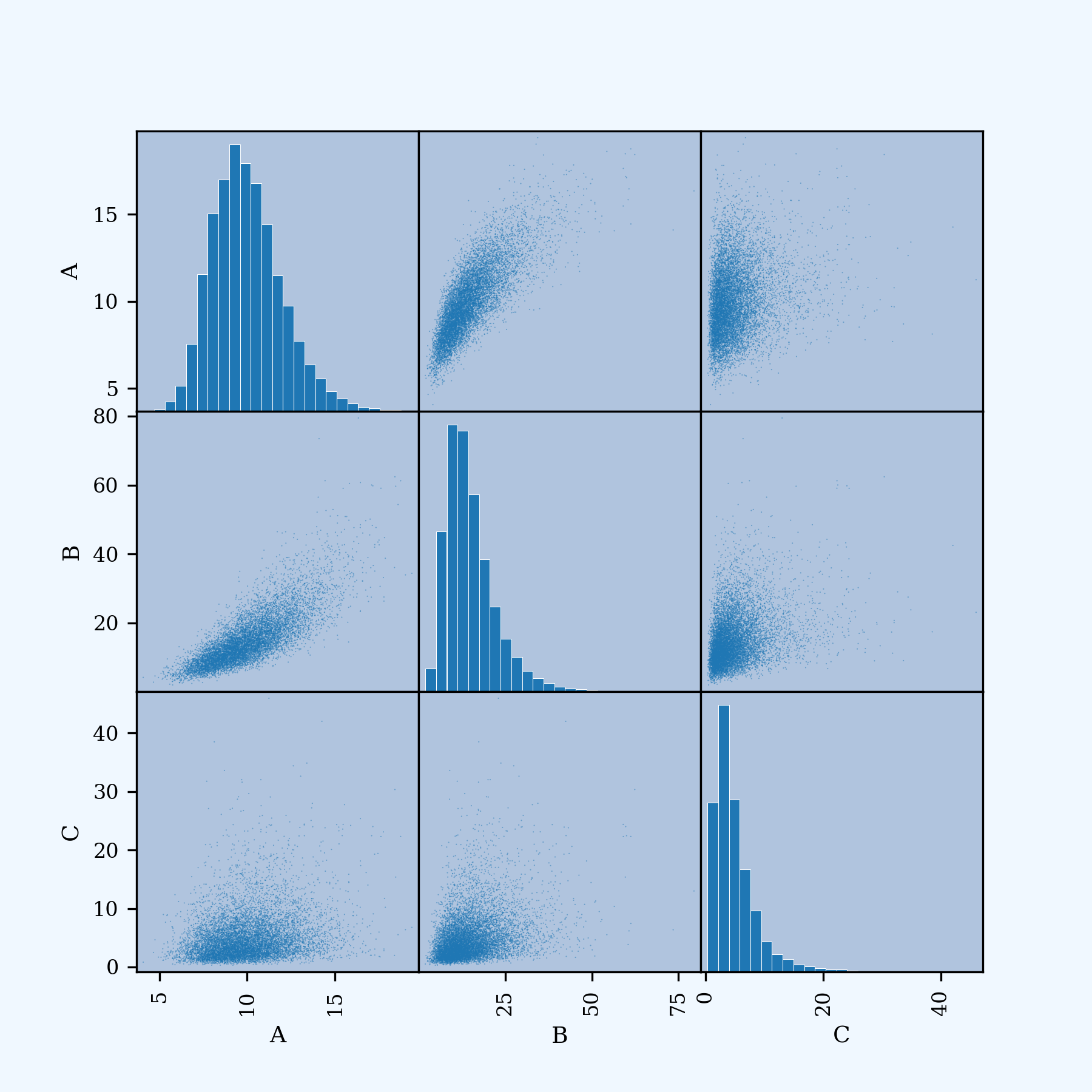
The sample uses a different random state and produces a different draw. Comparing
qdpoutput is one way to see if 10000 simulations is adequate. In this case there is good agreement.In [30]: qdp(df2) Out[30]: A B C total count 10000.000000 10000.000000 10000.000000 10000.000000 mean 9.991469 14.969470 4.987341 29.948280 std 1.997495 7.389115 3.910557 10.902512 min 4.070312 1.984375 0.304688 8.242188 25% 8.570312 9.742188 2.414062 22.304688 50% 9.789062 13.406250 3.906250 27.867188 75% 11.179688 18.351562 6.273438 35.460938 max 19.398438 79.468750 45.937500 111.164062 cv 0.199920 0.493612 0.784097 0.364045
2.12.4. Applying the Iman-Conover Algorithm
The method sample() automatically applies the Iman-Conover algorithm (described in The Iman-Conover Method). It is also easy to apply Iman-Conover to a dataframe using the method aggregate.utilities.iman_conover(). It reorders the input dataframe to have the same rank correlation as a multivariate normal reference sample with the desired linear correlation. Optionally, a multivariate t-distribution can be used as the reference.
Examples.
Apply Iman-Conover to the sample df with target the correlation rcm, reusing the variables created in the previous section. The achieved correlation is close to that requested, as shown in the last two blocks.
In [31]: from aggregate import iman_conover

In [32]: import pandas as pd

In [33]: ans = iman_conover(df[abc], rcm, add_total=False)

In [34]: qd(pd.DataFrame(rcm, index=abc, columns=abc))

        A       B       C
A       1 0.80331 0.24378
B 0.80331       1 0.35449
C 0.24378 0.35449       1

In [35]: qd(ans.corr())

        A       B       C
A       1 0.78111 0.22247
B 0.78111       1 0.31237
C 0.22247 0.31237       1
Setting the argument dof uses a t-copula reference with dof degrees of freedom. The t-copula with low degrees of freedom can produce pinched multivariate distributions. Use with caution.
In [36]: ans = iman_conover(df[abc], rcm, dof=2, add_total=False)

In [37]: qd(ans.corr())

        A       B       C
A       1 0.86152 0.51261
B 0.86152       1 0.49706
C 0.51261 0.49706       1

In [38]: scatter_matrix(ans, grid=False, figsize=(6, 6), diagonal='hist',
   ....:     hist_kwds={'density': True, 'bins': 25, 'lw': .25, 'ec': 'w'},
   ....:     s=1, marker='.');
   ....:

See WP REF for ways to apply Iman-Conover with different reference distributions.
Details. Creating the independent scores for Iman-Conover is quite time consuming. They are cached for a given sample size. Second and subsequent calls are far quicker (an order of magnitude) than the first call.
2.12.5. Applying the Re-Arrangement Algorithm
The method rearrangement_algorithm_max_VaR() implements the re-arrangement algorithm described in ../5_technical_guides/5_x_rearrangement_algorithm. It returns only the tail of the re-arrangement, since values below the requested percentile are irrelevant.
Apply to df and request 0.999-VaR. The marginals are the 10 largest values. The algorithm permutes them to balance large and small observations.
In [39]: from aggregate import rearrangement_algorithm_max_VaR

In [40]: ans = rearrangement_algorithm_max_VaR(df.iloc[:, :3], .999)

In [41]: qd(ans, float_format=fc)

         A        B        C    total
0    21.08    63.78    38.59   123.45
6    20.22    65.18    38.40   123.80
1    20.63    62.50    40.80   123.93
3    18.93    65.02    40.24   124.20
5    17.98    60.66    45.56   124.20
2    18.02    68.88    37.33   124.23
7    17.75    61.75    44.91   124.41
9    19.99    66.28    38.22   124.49
8    17.69    73.03    37.12   127.84
4    17.59    81.07    37.03   135.70
Here are the stand-alone sa VaRs by marginal, in total for df, in total for the correlated df2, and the re-arrangement solutions ra for a range of different percentiles. The column comon total shows VaR for the comonotonic sum of the marginals (which equals the largest TVaR and variance re-arrangement).
In [42]: ps = [9000, 9500, 9900, 9960, 9990, 9999]

In [43]: sa = pd.concat([df[c].sort_values().reset_index(drop=True).iloc[ps] for c in df]
   ....:                 +[df2.rename(columns={'total':'corr total'})['corr total'].\
   ....:                   sort_values().reset_index(drop=True).iloc[ps]], axis=1)
   ....:

In [44]: sa['comon total'] = sa[abc].sum(1)

In [45]: ra = pd.concat([rearrangement_algorithm_max_VaR(df.iloc[:, :3], p/10000).iloc[0]  for p in ps],
   ....:           axis=1, keys=ps).T
   ....:

In [46]: exhibit = pd.concat([sa, ra], axis=1, keys=['stand-alone', 're-arrangement'])

In [47]: exhibit.index = [f'{x/10000:.2%}' for x in exhibit.index]

In [48]: exhibit.index.name = 'percentile'

In [49]: qd(exhibit, float_format=fc)

           stand-alone                                                   re-arrangement           \
                     A        B        C    total corr total comon total              A        B
percentile
90.00%           12.59    24.75     9.73    41.48      44.22       47.06          15.64    28.69
95.00%           13.55    29.21    12.68    46.48      50.43       55.44          16.42    32.19
99.00%           15.45    39.98    20.55    58.15      65.26       75.98          17.75    44.51
99.60%           16.36    47.62    26.58    68.00      73.50       90.56          17.59    59.56
99.90%           17.59    60.66    37.03    80.20      93.51      115.28          21.08    63.78
99.99%           21.08    81.07    45.56   115.28     111.16      147.71          21.08    81.07


                  C    total
percentile
90.00%        12.70    57.02
95.00%        16.98    65.59
99.00%        26.37    88.62
99.60%        28.77   105.92
99.90%        38.59   123.45
99.99%        45.56   147.71
See also Worked Example.
2.12.6. Creating a Portfolio From a Sample
A Portfolio can be created from an existing sample by passing in a dataframe rather than a list of aggregates. This approach is useful when another model has created the sample, but the user wants to access other aggregate functionality. Each marginal in the sample is created as a dsev with the sampled outcomes. The p_total column used to set scenario probabilities if its is input, otherwise each scenario is treated as equally likely. The Portfolio ignores any the correlation structure of the sample; the marginals are treated as independent, but see Using Samples and the Switcheroo Trick for a way around this assumption.
Example.
Create a simple discrete sample from a three unit portfolio.
In [50]: sample = pd.DataFrame(
   ....:    {'A': [20, 22, 24, 6, 5, 6, 7, 8, 21, 3],
   ....:     'B': [20, 18, 16, 14, 12, 10, 8, 6, 4, 2],
   ....:     'C': [0, 0, 0, 0, 0, 0, 0, 0, 20, 40]})
   ....:

In [51]: qd(sample)

    A   B   C
0  20  20   0
1  22  18   0
2  24  16   0
3   6  14   0
4   5  12   0
5   6  10   0
6   7   8   0
7   8   6   0
8  21   4  20
9   3   2  40
Pass to Portfolio to create with these marginals. In this case, treat the marginals as discrete and update with bs=1.
In [52]: from aggregate import Portfolio

In [53]: p03 = Portfolio('Samp:03', sample)

In [54]: p03.update(bs=1, log2=8)

In [55]: qd(p03)

             E[X] Est E[X]    Err E[X]   CV(X) Est CV(X) Skew(X) Est Skew(X)
unit  X
A     Freq      1                            0
      Sev    12.2     12.2           0 0.65142   0.65142 0.37792     0.37792
      Agg    12.2     12.2           0 0.65142   0.65142 0.37792     0.37792
B     Freq      1                            0
      Sev      11       11           0 0.52223   0.52223       0           0
      Agg      11       11           0 0.52223   0.52223       0           0
C     Freq      1                            0
      Sev       6        6 -3.3307e-16  2.1344    2.1344  1.9198      1.9198
      Agg       6        6 -3.3307e-16  2.1344    2.1344  1.9198      1.9198
total Freq      3                            0
      Sev  9.7333   9.7333           0 0.99572            1.0775
      Agg    29.2     29.2 -3.3307e-16 0.55238   0.55238  1.0061      1.0061
log2 = 8, bandwidth = 1, validation: not unreasonable.
The univariate statistics for each marginal are the same as the sample input, but because they added independently, the totals differ. The sample has negative correlation and a lower CV.
In [56]: sample['total'] = sample.sum(1)

In [57]: qdp(sample)
Out[57]:
               A          B          C      total
count  10.000000  10.000000  10.000000  10.000000
mean   12.200000  11.000000   6.000000  29.200000
std     7.947327   5.744563  12.806248  12.998461
min     3.000000   2.000000   0.000000  14.000000
25%     6.000000   6.500000   0.000000  16.250000
50%     7.500000  11.000000   0.000000  30.000000
75%    20.750000  15.500000   0.000000  40.000000
max    24.000000  20.000000  40.000000  45.000000
cv      0.651420   0.522233   2.134375   0.445153
The Portfolio total is a convolution of the input marginals and includes all possible combinations added independently. The figure plots the distribution functions.
In [58]: ax = p03.density_df.filter(regex='p_[ABCt]').cumsum().plot(
   ....:     drawstyle='steps-post', lw=1, figsize=(3.5, 2.45))
   ....:

In [59]: ax.plot(np.hstack((0, sample.total.sort_values())), np.linspace(0, 1, 11),
   ....:     drawstyle='steps-post', lw=2, label='dependent');
   ....:

In [60]: ax.set(xlim=[-2, 90]);

In [61]: ax.legend(loc='lower right');

2.12.7. Using Samples and the Switcheroo Trick
Portfolio objects created from a sample ignore the dependency structure; the aggregate convolution algorithm always assumes independence. It is highly desirable to retain the sample’s dependency structure. Many calculations rely only on \(\mathsf E[X_i\mid X]\) and not the input densities per se. Thus, we reflect dependency if we alter the values \(\mathsf E[X_i\mid X]\) based on a sample and recompute everything that depends on them. The method Portfolio.add_exa_sample() implements this idea.
Example.
sample was chosen to have lots of ties - different ways of obtaining the same total outcome.
In [62]: qd(sample)

    A   B   C  total
0  20  20   0     40
1  22  18   0     40
2  24  16   0     40
3   6  14   0     20
4   5  12   0     17
5   6  10   0     16
6   7   8   0     15
7   8   6   0     14
8  21   4  20     45
9   3   2  40     45
Apply add_exa_sample to the sample dataframe and look at the outcomes with positive probability. When a total outcome can occur in multiple ways, exeqa_i gives the average value of unit i.
The function is applied to a copy of the original Portfolio object because it invalidates various internal states. The output dataframe is indexed by total loss. Notice that rows sum to the correct total.
In [63]: p03sw = Portfolio('Samp:03sw', sample)

In [64]: p03sw.update(bs=1, log2=8)

In [65]: df = p03sw.add_exa_sample(sample)

In [66]: qd(df.query('p_total > 0').filter(regex='p_total|exeqa_[ABC]'))

      p_total  exeqa_A  exeqa_B  exeqa_C
14.0      0.1        8        6        0
15.0      0.1        7        8        0
16.0      0.1        6       10        0
17.0      0.1        5       12        0
20.0      0.1        6       14        0
40.0      0.3       22       18        0
45.0      0.2       12        3       30
Swap the density_df dataframe — the switcheroo trick.
In [67]: p03sw.density_df = df
See the function Portfolio.create_from_sample for a single step create from sample, update, add exa calc, and switcheroo.
Most Portfolio spectral functions depend only on marginal conditional expectations. Applying these functions through p03sw reflects dependencies. Calibrate some distortions to a 15% return. The maximum loss is only 45, so use a 1-VaR, no default capital standard.
In [68]: p03sw.calibrate_distortions(ROEs=[0.15], Ps=[1], strict='ordered');

In [69]: qd(p03sw.distortion_df)

                      S    L      P     PQ      Q  COC   param  std_param       error
a    LR       method
45.0 0.934075 ccoc    0 29.2 31.261 2.2753 13.739 0.15    0.15    0.13043           0
              ph      0 29.2 31.261 2.2753 13.739 0.15 0.80913     0.1055  4.1444e-09
              wang    0 29.2 31.261 2.2753 13.739 0.15 0.18223    0.10253 -1.6102e-07
              dual    0 29.2 31.261 2.2753 13.739 0.15   1.228    0.10234 -9.8354e-08
              tvar    0 29.2 31.261 2.2753 13.739 0.15 0.12059    0.12059   5.935e-06
Apply the PH and dual to the independent and dependent portfolios. Asset level 45 is the 0.861 percentile of the independent.
In [70]: d1 = p03sw.dists['ph']; d2 = p03sw.dists['dual']

In [71]: for d in [d1, d2]:
   ....:     print(d.name)
   ....:     print('='*74)
   ....:     pr = p03.price(1, d)
   ....:     pr45 = p03.price(.861, d)
   ....:     prsw = p03sw.price(1, d)
   ....:     a = pd.concat((pr.df, pr45.df, prsw.df), keys=['pr', 'pr45', 'prsw'])
   ....:     qd(a, float_format=lambda x: f'{x:7.3f}')
   ....:
ph
==========================================================================

statistic                   L       P       M       Q       a      LR      PQ     COC
     distortion unit
pr   ph         A      12.200  12.944   0.744  13.129  26.073   0.943   0.986   0.057
                B      11.000  11.376   0.376   9.544  20.919   0.967   1.192   0.039
                C       6.000   8.400   2.400  28.608  37.008   0.714   0.294   0.084
                total  29.200  32.719   3.519  51.281  84.000   0.892   0.638   0.069
pr45 ph         A      11.675  12.059   0.384   3.624  15.682   0.968   3.328   0.106
                B      10.578  10.674   0.096   2.160  12.834   0.991   4.941   0.045
                C       4.803   6.457   1.654  10.027  16.484   0.744   0.644   0.165
                total  27.055  29.189   2.134  15.811  45.000   0.927   1.846   0.135
prsw ph         A      12.200  12.571   0.371   3.371  15.942   0.970   3.729   0.110
                B      11.000  10.532  -0.468  -0.187  10.345   1.044 -56.386   2.507
                C       6.000   8.158   2.158  10.555  18.713   0.736   0.773   0.204
                total  29.200  31.261   2.061  13.739  45.000   0.934   2.275   0.150
dual
==========================================================================

statistic                   L       P       M       Q       a      LR      PQ     COC
     distortion unit
pr   dual       A      12.200  13.061   0.861  15.011  28.071   0.934   0.870   0.057
                B      11.000  11.523   0.523  11.590  23.113   0.955   0.994   0.045
                C       6.000   7.171   1.171  25.645  32.816   0.837   0.280   0.046
                total  29.200  31.754   2.554  52.246  84.000   0.920   0.608   0.049
pr45 dual       A      11.675  12.422   0.747   5.480  17.902   0.940   2.267   0.136
                B      10.578  11.009   0.432   4.186  15.195   0.961   2.630   0.103
                C       4.803   5.716   0.914   6.187  11.903   0.840   0.924   0.148
                total  27.055  29.148   2.093  15.852  45.000   0.928   1.839   0.132
prsw dual       A      12.200  12.874   0.674   4.947  17.821   0.948   2.602   0.136
                B      11.000  11.197   0.197   2.644  13.840   0.982   4.235   0.074
                C       6.000   7.191   1.191   6.148  13.339   0.834   1.170   0.194
                total  29.200  31.261   2.061  13.739  45.000   0.934   2.275   0.150
2.12.8. Summary of Objects Created by DecL
Objects created by build() in this guide. Objects created directly by class constructors are not entered into the knowledge database.
In [72]: from aggregate import pprint_ex

In [73]: for n, r in build.qlist('^Samp:').iterrows():
   ....:     pprint_ex(r.program, split=20)
   ....:
agg Samp:01
  1 claim
  sev lognorm 10 cv .4
  fixed
port Samp:02
  agg A
    1 claim
    sev lognorm 10 cv .2
    fixed
  agg B
    1 claim
    sev lognorm 15 cv .5
    fixed
  agg C
    1 claim
    sev lognorm 5 cv .8
    fixed