2.3. A Ten Minute Guide to aggregate
Objectives: A whirlwind introduction—don’t expect to understand everything the first time, but you will see what you can achieve with the package. Follows the pandas model, a long 10 minutes.
Audience: A new user.
Prerequisites: Python programming; aggregate distributions. Read in conjunction with Student or Actuarial Student practice guides.
See also: API Reference, The Dec Language.
Contents:
-
-
Estimating Bucket Size for Discretization
Methods and Properties Common To Aggregate and Portfolio Classes
-
2.3.1. Principle Classes
The aggregate package makes working with aggregate probability distributions as straightforward as working with parametric distributions even though their densities rarely have closed-form expressions. It is built around five principal classes.
The
Underwriterclass keeps track of everything in itsknowledgedataframe, interprets Dec Language (DecL, pronounced like deckle, /ˈdɛk(ə)l/) programs, and acts as a helper.The
Severityclass models a size of loss distribution (a severity curve).The
Aggregateclass models a single unit of business, such as a line, business unit, geography, or operating division.The
Distortionclass provides a distortion function, the basis of a spectral risk measure.The
Portfolioclass models multiple units. It extends the functionality inAggregate, adding pricing, calibration, and allocation capabilities.
There is also a Frequency class that Aggregate derives from, but it is rarely used standalone, and a Bounds class for advanced users.
2.3.2. The Underwriter Class
The Underwriter class is an interface into the computational functionality of aggregate. It does two things:
Creates objects using the DecL language, and
Maintains a library of DecL object specifications called the knowledge. New objects are automatically added to the knowledge.
To get started, import build, a pre-configured Underwriter and qd(), a quick-display function. Import the usual suspects too, for good measure.
In [1]: from aggregate import build, qd

In [2]: import pandas as pd, numpy as np, matplotlib.pyplot as plt
Printing build reports its name, the number of objects in its knowledge, and other information about hyper-parameter default values. site_dir is where various outputs will be stored. default_dir is for internal package data. The build object loads an extensive test suite of DecL programs with over 130 entries.
In [3]: build
Out[3]:
underwriter        Rory
version            0.30.1
knowledge          146 programs
update             True
log2               16
debug              False
validation_eps     0.0001
site dir           ~/aggregate/databases
default dir        ~/checkouts/readthedocs.org/user_builds/aggregate/checkouts/latest/aggregate/agg

help
build.knowledge    list of all programs
build.qshow(pat)   show programs matching pattern
build.show(pat)    build and display matching pattern
2.3.2.1. Object Creation Using DecL and build()
The Underwriter class interprets DecL programs (The Dec Language). These allow severities, aggregates and portfolios to be created using standard insurance language.
For example, to build an Aggregate using DecL and report key statistics for frequency, severity, and aggregate, needs just two commands.
In [4]: a01 = build('agg TenM:01 100 claims 100 xs 0 sev lognorm 10 cv 1.25 poisson')

In [5]: qd(a01)

      E[X] Est E[X]    Err E[X]   CV(X) Est CV(X)  Skew(X) Est Skew(X)
X
Freq   100                          0.1                0.1
Sev  9.918    9.918  2.8323e-10  1.1639    1.1639   3.4165      3.4165
Agg  991.8    991.8 -4.5177e-10 0.15345   0.15345  0.28923     0.28923
log2 = 16, bandwidth = 1/32, validation: not unreasonable.
DecL is supposed to be human-readable, so I hope you can guess the meaning of the DecL code (TenM:01 is just a label):
agg TenM:01 5 claims 1000 xs 0 sev lognorm 50 cv 4 poisson
The units are 1000s of USD, EUR, or GBP.
DecL is a custom language, created to describe aggregate distributions. Alternatives are to use positional arguments or key word arguments in function calls. The former are confusing because there are so many. The latter are verbose, because of the need to specify the parameter name. DecL is a concise, expressive, flexible, and powerful alternative.
2.3.2.2. Important: Formatting a DecL Program
Important
All DecL programs are one line long.
It is best to break a DecL program up to make it more readable. The fact that Python automatically concatenates strings between parenthesis makes this easy. The program above is always entered in the help as:
a01 = build('agg TenM:01 '
            '100 claims '
            '100 xs 0 '
            'sev lognorm 10 cv 1.25 '
            'poisson')
which Python makes equivalent to:
a01 = build('agg TenM:01 100 claims 100 xs 0 sev lognorm 10 cv 1.25 poisson')
as originally entered. Pay attention to spaces at the end of each line! Entering:
a01 = build('agg TenM:01'
            '100 claims'
            '100 xs 0'
            'sev lognorm 10 cv 1.25'
            'poisson')
produces:
a01 = build('agg TenM:01100 claims100 xs 0sev lognorm 10 cv 1.25poisson')
which results in syntax errors.
DecL includes a Python newline \. All programs in the help are entered so they can be cut and pasted.
2.3.2.3. Object Creation from the Knowledge Database
The knowledge dataframe is a database of DecL programs and a parsed
dictionaries to create objects. build loads an extensive library by
default. Users can create and load their own databases, allowing them to share common parameters for
severity (size of loss) curves,
aggregate distributions (e.g., industry losses in major classes of business, or total catastrophe losses from major perils), and
portfolios (e.g., an insurer’s reference portfolio or educational examples like Bodoff’s examples and Pricing Insurance Risk case studies).
It is indexed by object kind (severity, aggregate, portfolio) and name, and accessed as the read-only property build.knowledge. Here are the first five rows of the knowledge loaded by build.
In [6]: qd(build.knowledge.head(), justify="left", max_colwidth=60)

              program                                                       \
kind name
agg  A.Dice00  agg A.Dice00 dfreq  [1:6]  dsev  [1]  note{The roll of a...
     A.Dice01  agg A.Dice01 dfreq  [1]  dsev  [1:6]  note{Same as previ...
     A.Dice02  agg A.Dice02 dfreq  [2]  dsev  [1:6]  note{Sum of the ro...
     A.Dice03  agg A.Dice03 dfreq  [5]  dsev  [1:6]  note{Sum of the ro...
     A.Dice04  agg A.Dice04 dfreq  [1:6]  dsev  [1:6]  note{Sum of a di...

              spec
kind name
agg  A.Dice00  {'name': 'A.Dice00', 'freq_name': 'empirical', 'freq_a':...
     A.Dice01  {'name': 'A.Dice01', 'freq_name': 'empirical', 'freq_a':...
     A.Dice02  {'name': 'A.Dice02', 'freq_name': 'empirical', 'freq_a':...
     A.Dice03  {'name': 'A.Dice03', 'freq_name': 'empirical', 'freq_a':...
     A.Dice04  {'name': 'A.Dice04', 'freq_name': 'empirical', 'freq_a':...
A row in the knowledge can be accessed by name using build. This example models the roll of a single die.
In [7]: print(build['A.Dice00'])
kind                	agg
name                	A.Dice00
spec                	<class 'dict'>
program             	agg A.Dice00 dfreq  [1:6]  dsev  [1]  note{The roll of a single dice.}
object              	<class 'NoneType'>
The argument 'A.Dice00' is passed through to the underlying dataframe’s getitem.
A row in the knowledge can be created as a Python object using:
In [8]: aDice = build('A.Dice00')

In [9]: qd(aDice)

      E[X] Est E[X]   Err E[X]   CV(X) Est CV(X) Skew(X) Est Skew(X)
X
Freq   3.5                     0.48795                 0
Sev      1        1          0       0         0
Agg    3.5      3.5 4.4409e-16 0.48795   0.48795       0    4.85e-14
log2 = 4, bandwidth = 1, validation: not unreasonable.
The argument in this case is passed through to the method Underwriter.build(), which first looks for A.Dice00 in the knowledge. If it fails, it tries to interpret its argument as a DecL program.
The method build.qlist() (quick list) searches the knowledge using a regex (regular expression) applied to the names, and returning a dataframe of specifications. build.qshow() (quick show) just displays them.
In [10]: build.qshow('Dice')

                program
name
A.Dice00         agg A.Dice00 dfreq  [1:6]  dsev  [1]  note{The roll of a single dice.}
A.Dice01         agg A.Dice01 dfreq  [1]  dsev  [1:6]  note{Same as previous example.}
A.Dice02         agg A.Dice02 dfreq  [2]  dsev  [1:6]  note{Sum of the rolls of two dice.}
A.Dice03         agg A.Dice03 dfreq  [5]  dsev  [1:6]  note{Sum of the rolls of five dice.}
A.Dice04         agg A.Dice04 dfreq  [1:6]  dsev  [1:6]  note{Sum of a dice roll of dice rolls}
A.Dice05         agg A.Dice05 dfreq  [1:4]  dsev  [1:16]  note{Something you can't do easily by hand}
The method build.show() also searches the knowledge using a regex applied to the names, but it creates and plots each match by default. Be careful not to create too many objects! Try running:
build.show('Dice')
Add argument return_df=True to return a list of created objects and a dataframe containing information about each.
2.3.2.4. Underwriter Behind the Scenes
This section should be skipped the first time through.
Each object has a kind property and a name property, and it can be manifest as a DecL program, a dictionary specification, or a Python class instance. The class can be updated or not updated. In detail:
kind equals sev for a
Severity, agg for aAggregate, port for aPortfolio, and distortion for aDistortion(dist could be distribution);name is assigned to the object by the user; it is different from the Python variable name holding the object;
spec is a (derived) dictionary specification;
program is the DecL program as a text string; and
object is the actual Python object, an instance of a class.
Underwriter.write() is a low-level creator function. It takes a DecL program or knowledge item name as input.
It searches the knowledge for the argument and returns it if it finds one object. It throws an error if the name is not unique. If the name is not in the knowledge it continues.
It calls
Underwriter.interpret_program()to pre-process the DecL and then lex and parse it one line at a time.It looks up occurrences of
sev.ID,agg.ID(IDis an object name) in the knowledge and replaces them with their definitions.It calls
Underwriter.factory()to create any objects and update them if requested.It returns a list of
Answerobjects, with kind, name, spec, program, and object attributes.
Underwriter.write_file() reads a file and passes it to Underwriter.write(). It is a convenience function.
The Underwriter.build() method wraps the
Underwriter.write() and provides sensible defaults to shield the user from its internal details. \(build\) takes the following steps:
It calls
write()withupdate=False.It then estimates sensible hyper-parameters and uses them to
update()the object’s discrete distribution. It tries to distinguish discrete output distributions from continuous or mixed ones.If the DecL program produces only one output, it strips it out of the answer returned by
writeand returns just that object.If the DecL program produces only one portfolio output (but possibly other non-portfolio objects), it returns just that.
Underwriter.interpret_program() interprets DecL programs and matches them with the parsed specs in an Answer(kind, name, spec, program, object=None) object. It adds the result to the knowledge.
Underwriter.factory() takes an Answer argument and updates it by creating the relevant object and updating it if build.update is True.
A set of methods called interpreter_xxx() run DecL programs through parser for debugging purposes, but do not create any output or add anything to the knowledge.
Underwriter.interpreter_line()works on one line.Underwriter.interpreter_file()works on each line in a file.Underwriter.interpreter_list()works on each item in a list.Underwriter._interpreter_work()does the actual parsing.
2.3.3. How aggregate Represents Distributions
A distribution is represented as a discrete numerical approximation. To “know or compute a distribution” means that we have a discrete stair-step approximation to the true distribution function that jumps (is supported) only on integer multiples of a fixed bandwidth or bucket size \(b\) (called bs in the code). The distribution is represented by \(b\) and a vector of probabilities \((p_0,p_1,\dots, p_{n-1})\) with the interpretation
All subsequent computations assume that this approximation is the distribution. For example, moments are estimated using
See Digital Representation of Distributions for more details.
2.3.4. The Severity Class
The Severity class derives from scipy.stats.rv_continuous, see scipy help. It contains a member stats.rv_continuous variable fz that is the ground-up unlimited severity and it adds support for limits and attachments. For example, the cdf function is coded:
def _cdf(self, x, *args):
    if self.conditional:
        return np.where(x >= self.limit, 1,
            np.where(x < 0, 0,
                     (self.fz.cdf(x + self.attachment) -
                     (1 - self.pattach)) / self.pattach))
    else:
        return np.where(x < 0, 0,
            np.where(x == 0, 1 - self.pattach,
                 np.where(x > self.limit, 1,
                      self.fz.cdf(x + self.attachment, *args))))
Severity can determine its shape parameter from a CV analytically for lognormal, gamma, inverse gamma, and inverse Gaussian distributions, and attempts to use a Newton-Raphson method to determine it for all other one-shape parameter distributions. (The CV is adjusted using the scale factor for zero parameter distributions.) Once the shape is known, it uses scaling to produce the required mean. Warning: The numerical methods are not always reliable.
Severity computes layer moments analytically for the lognormal, Pareto, and gamma, and uses numerical integration of the quantile function (isf) for all other distributions. These estimates can become unreliable for very thick tailed distributions. It uses self.fz.stats('mvs') and the object limit to determine if the requested moment actually exists before attempting numerical integration.
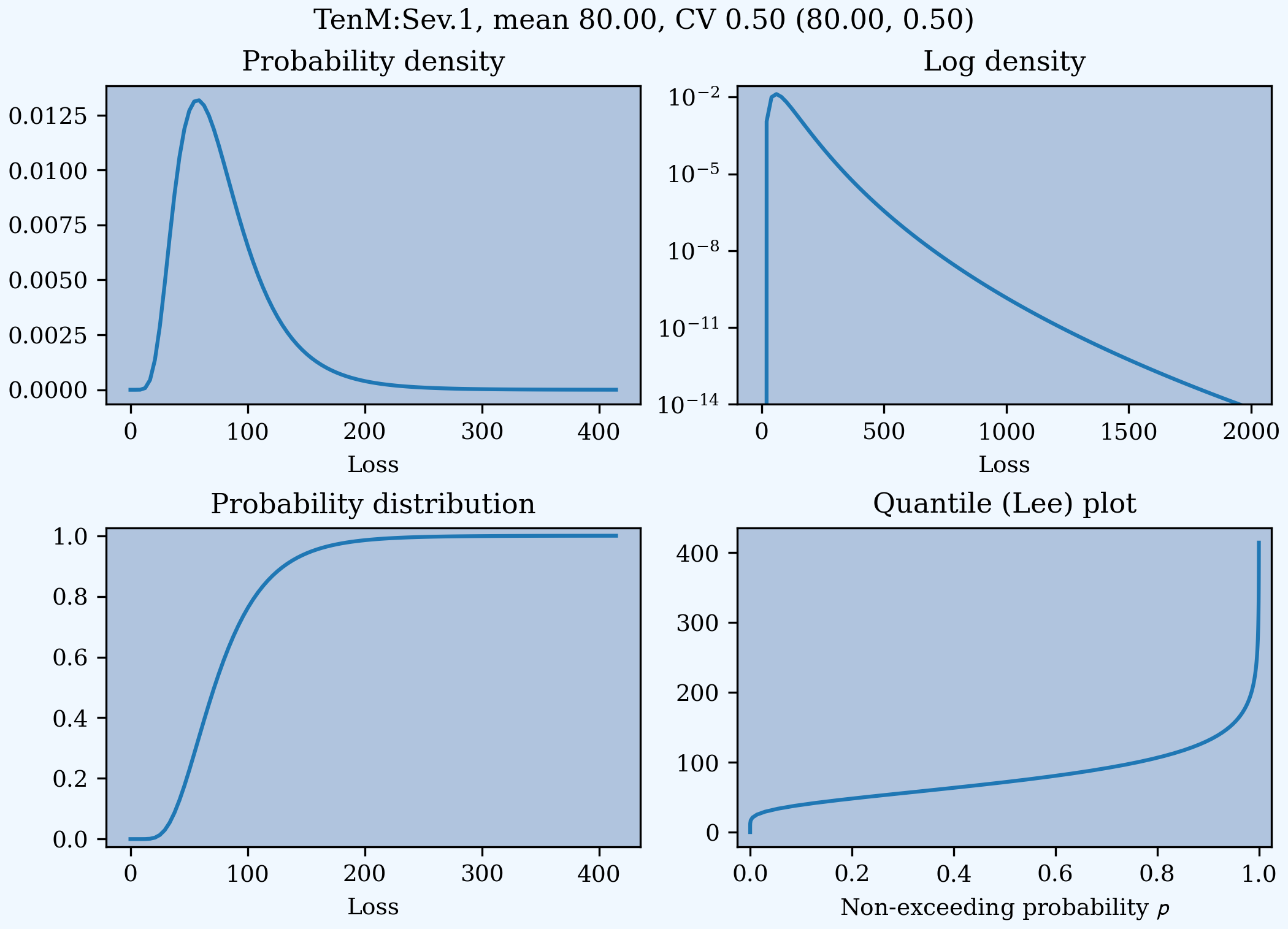
Severity has a plot() method that graphs the density, log density, cdf, and quantile (Lee) functions.
A Severity can be created using DecL using any of the following five forms.
sev NAME sev.BUILDIN_IDis a knowledge lookup forBUILTIN_IDsev NAME DISTNAME SHAPE1 <SHAPE2>whereDISTAMEis the name of anyscipy.statscontinuous random variable with zero, one, or two shape parameters, see the DecL/list of distributions.sev NAME SCALE * DISTNAME SHAPE1 <SHAPE2> + LOCsev NAME DISTNAME MEAN cv CVsev NAME SCALE * DISTNAME MEAN cv CV + LOCorsev NAME SCALE * DISTNAME MEAN cv CV - LOC
Either or both of SCALE and LOC can be present. In the mean and CV form, the mean refers to the unshifted, unscaled mean, but the CV refers to the shifted and scaled CV — because you usually want to control the overall CV.
Example.
lognorm 80 cv 0.5 results in an unshifted lognormal with mean 80 and CV 0.5.
In [11]: s0 = build(f'sev TenM:Sev.1 '
   ....:             'lognorm 80 cv .5')
   ....:

In [12]: mf, vf = s0.fz.stats(); m, v = s0.stats()

In [13]: s0.plot(figsize=(2*3.5, 2*2.45+0.15), layout='AB\nCD');

In [14]: plt.gcf().suptitle(f'{s0.name}, mean {m:.2f}, CV {v**.5/m:.2f} ({mf:.2f}, {vf**.5/mf:.2f})');

In [15]: print(m,v,mf,vf)
80.00000000000004 1599.9999999999936 80.00000000000001 1600.0000000000002
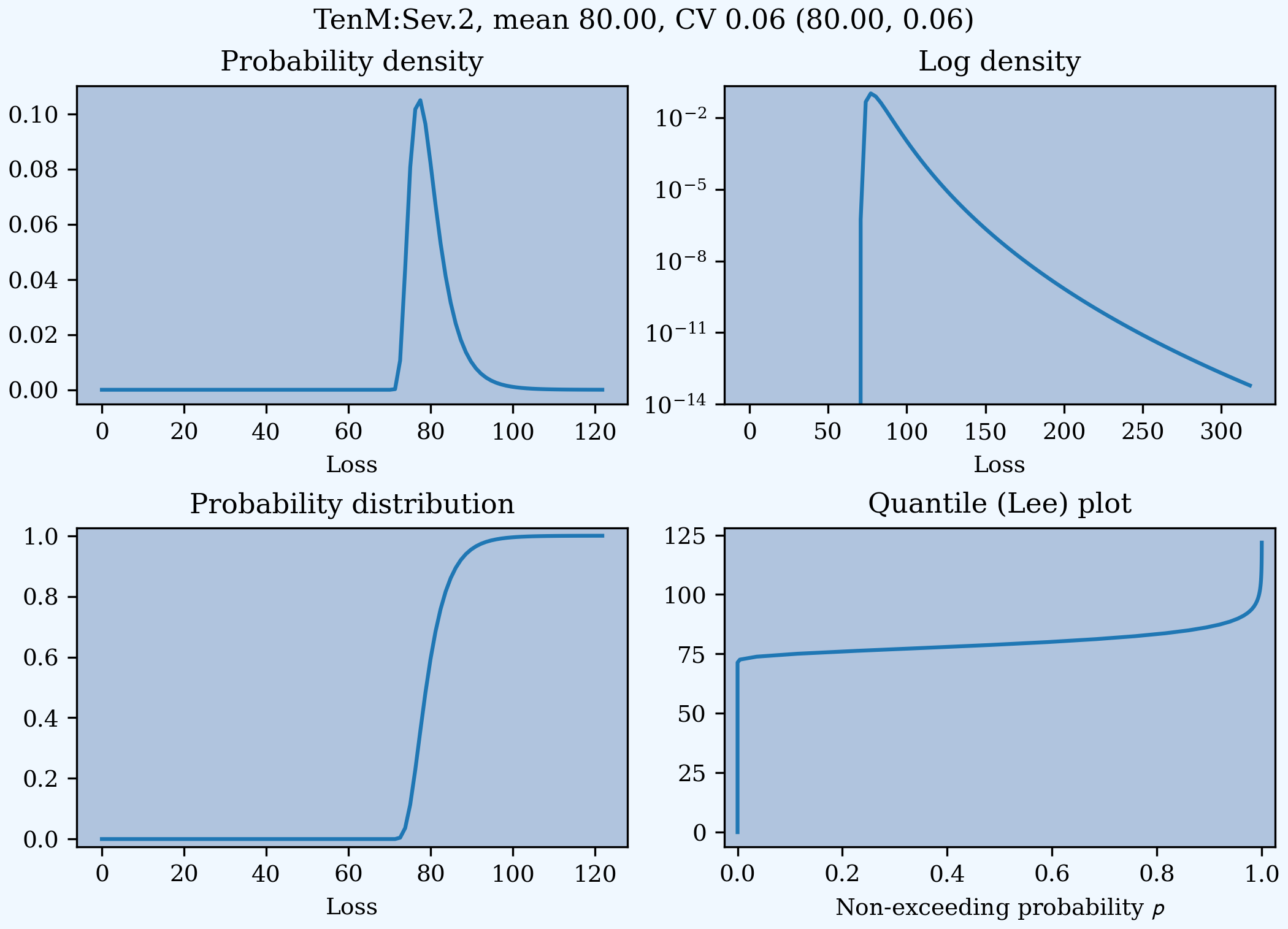
Combining scaling, shifts, and mean/cv entry like so 10 * lognorm 1 cv 0.5 + 70 results in a distribution with mean 10 * 1 + 70 = 80, a standard deviation of 10 * 0.5 = 5, and a cv of 5 / 80.
In [16]: s1 = build(f'sev TenM:Sev.2 '
   ....:             '10 * lognorm 1 cv .5 + 70')
   ....:

In [17]: mf, vf = s1.fz.stats(); m, v = s1.stats()

In [18]: s1.plot(figsize=(2*3.5, 2*2.45+0.15), layout='AB\nCD');

In [19]: plt.gcf().suptitle(f'{s1.name}, mean {m:.2f}, CV {v**.5/m:.2f} ({mf:.2f}, {vf**.5/mf:.2f})');

In [20]: print(m,v,mf,vf)
80.00000002527862 25.000006201477845 80.0 25.000000000000004
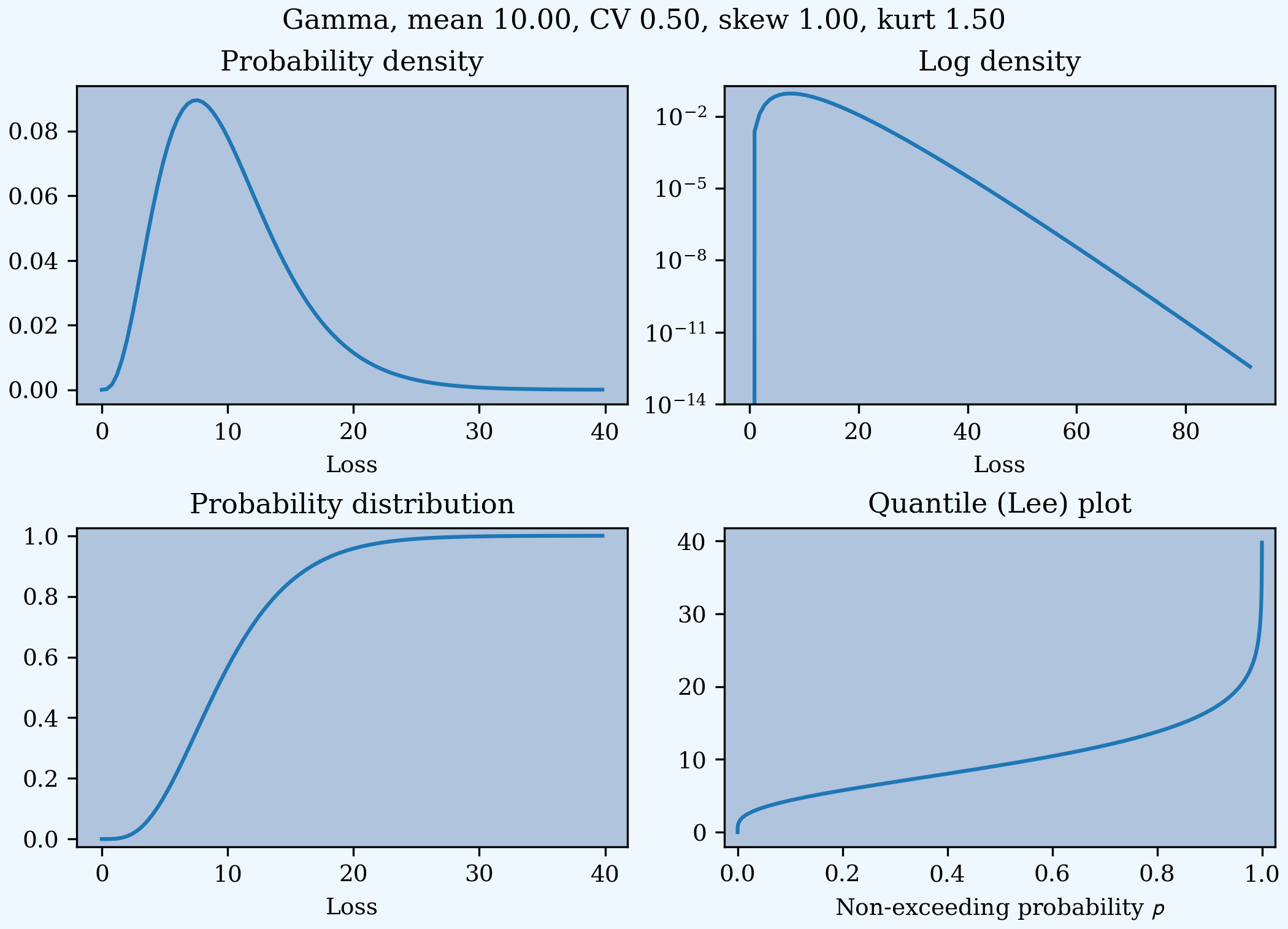
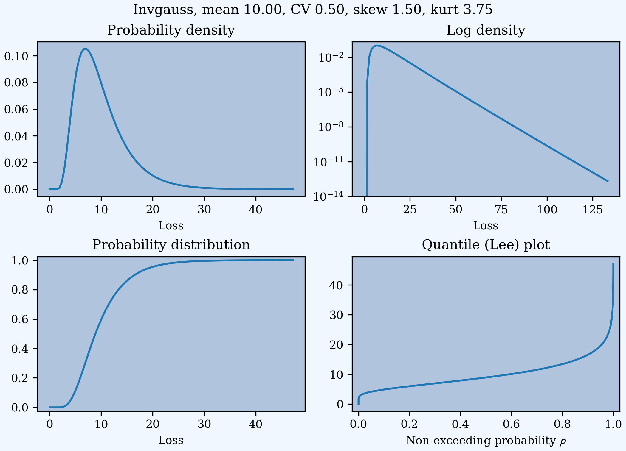
Examples.
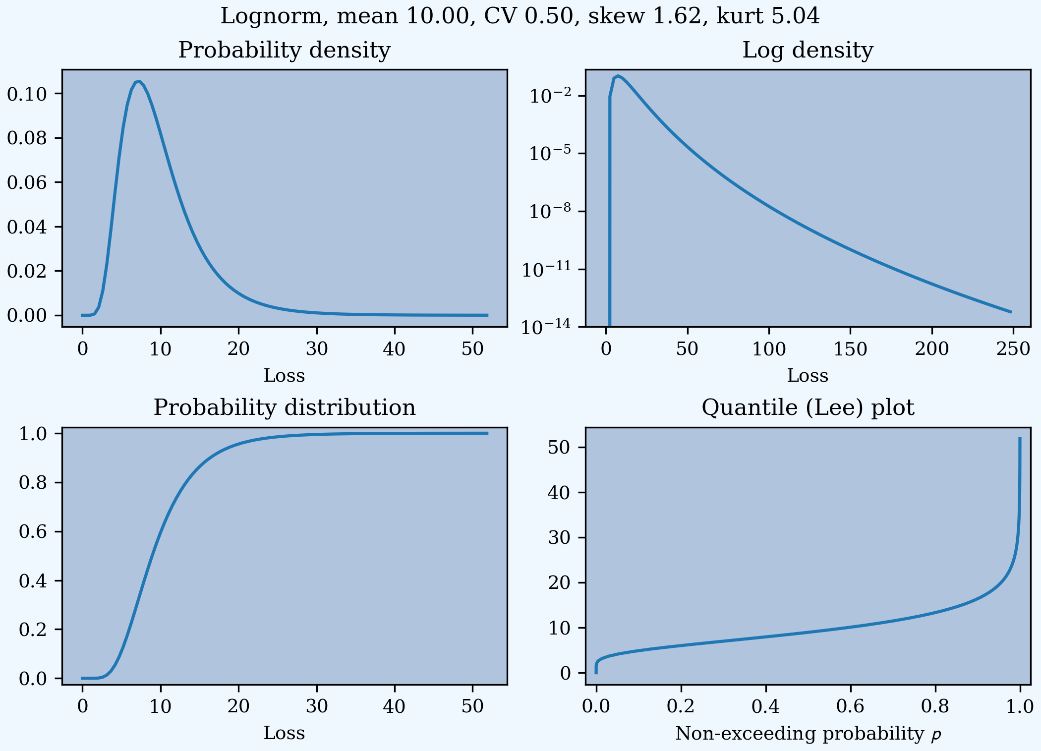
This example compares the shapes of gamma, inverse Gaussian, lognormal, and inverse gamma severities with the same mean and CV. First, a short function to create the examples.
In [21]: def plot_example(dist_name):
   ....:     s = build(f'sev TenM:{dist_name.title()} '
   ....:               f'{dist_name} 10 cv .5')
   ....:     m, v, sk, k = s.fz.stats('mvsk')
   ....:     s.plot(figsize=(2*3.5, 2*2.45+0.15), layout='AB\nCD')
   ....:     plt.gcf().suptitle(f'{dist_name.title()}, mean {m:.2f}, '
   ....:                        f'CV {v**.5/m:.2f}, skew {sk:.2f}, kurt {k:.2f}')
   ....:
Execute on the desired distributions.
In [22]: plot_example('gamma')

In [23]: plot_example('invgauss')

In [24]: plot_example('lognorm')

In [25]: plot_example('invgamma')

Examples.
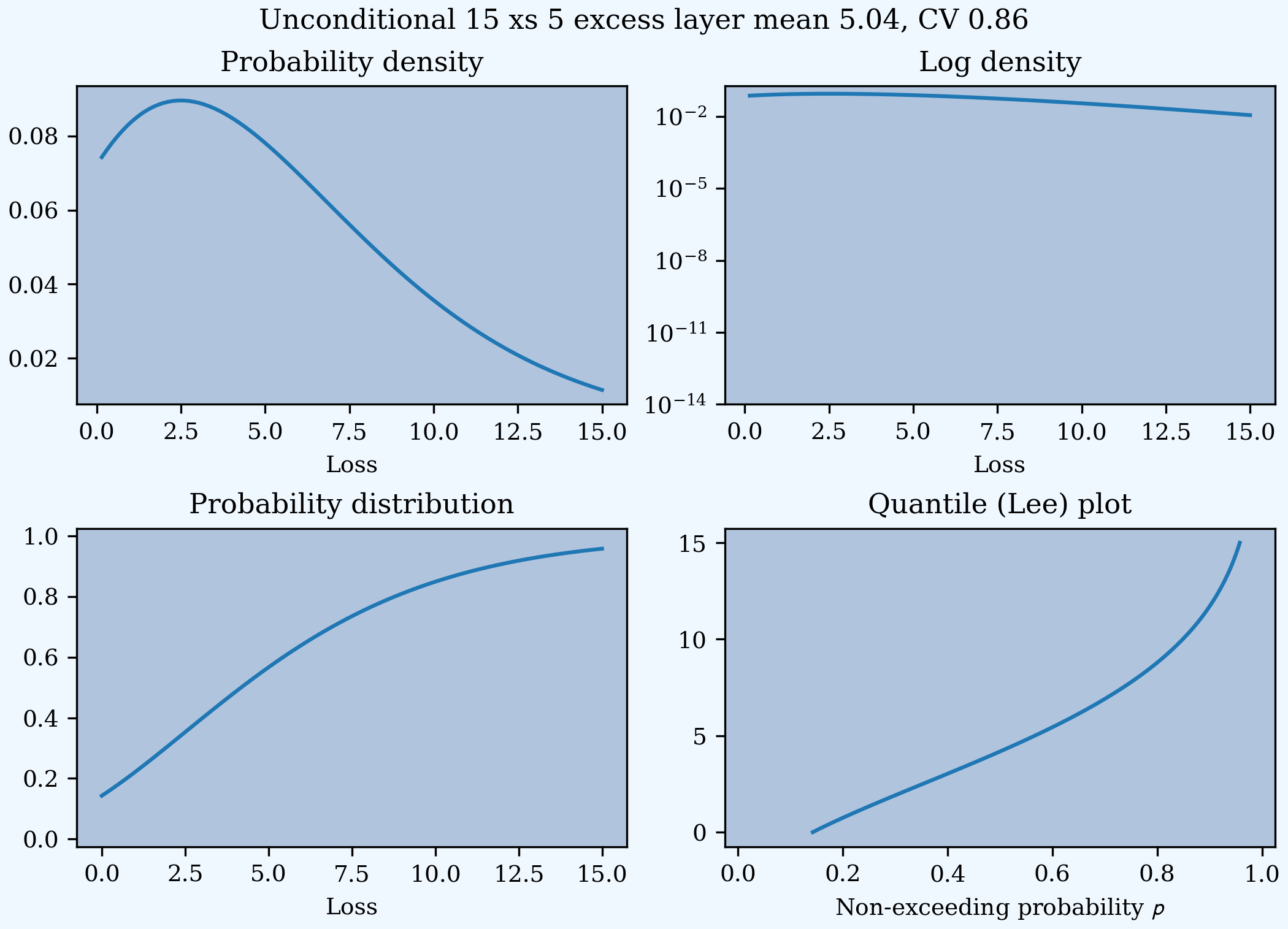
This example show the impact of adding a limit and attachment.
Limits and attachments determine exposure in DecL and they belong to the Aggregate specification. DecL cannot be used to set the limit and attachment of a Severity object. One way to apply them is to create an aggregate with a fixed frequency of one claim. By default, the severity is conditional on a loss to the layer.
In [26]: limit, attach = 15, 5

In [27]: s2 = build(f'agg TenM:SevLayer 1 claim {limit} xs {attach} sev gamma 10 cv .5 fixed')

In [28]: m, v, sk, k = s2.sevs[0].fz.stats('mvsk')

In [29]: s2.sevs[0].plot(n=401, figsize=(2*3.5, 2*2.45+0.3), layout='AB\nCD')

In [30]: plt.gcf().suptitle(f'Ground-up severity\nGround-up gamma mean {m:.2f}, CV {v**0.5/m:.2f}, skew {sk:.2f}, kurt {k:.2f}\n'
   ....:                    f'{limit} xs {attach} excess layer mean {s2.est_m:.2f}, CV {s2.est_cv:.2f}, skew {s2.est_skew:.2f}, kurt {k:.2f}');
   ....:

A Severity can be created directly using args and kwargs. Here is an example. It also shows the impact of making the severity unconditional (on a loss to the layer). Start by creating the conditional (default) severity and plotting it.
In [31]: from aggregate import Severity

In [32]: s3 = Severity('gamma', attach, limit, 10, 0.5)

In [33]: s3.plot(n=401, figsize=(2*3.5, 2*2.45+0.15), layout='AB\nCD')

In [34]: m, v = s3.stats()

In [35]: plt.gcf().suptitle(f'{limit} xs {attach} excess layer mean {m:.2f}, CV {v**.5/m:.2f}');
Next, create an unconditional version. The lower pdf is scaled down by the probability of attaching the layer, and the left end of the cdf shifted up by the probability of not attaching the layer. These probabilities are given by the underlying fz object’s sf and cdf.
In [36]: s4 = Severity('gamma', attach, limit, 10, 0.5, sev_conditional=False)

In [37]: s4.plot(figsize=(2*3.5, 2*2.45+0.15), layout='AB\nCD')

In [38]: m, v = s4.stats()

In [39]: plt.gcf().suptitle(f'Unconditional {limit} xs {attach} excess layer mean {m:.2f}, CV {v**.5/m:.2f}');

In [40]: print(f'Probability of attaching layer {s4.fz.cdf(attach):.3f}')
Probability of attaching layer 0.143
Although Severity accepts a weight argument, it does not actually support weighted severities. It models only one component. Aggregate handles weighted severities by creating a separate Severity for each component.
2.3.5. The Aggregate Class
2.3.5.1. Creating an Aggregate Distribution
Aggregate objects can be created in three ways:
Generally, they are created using DecL by
Underwriter.build(), as shown in Object Creation Using DecL and build().Objects in the knowledge can be created by name.
Advanced users and programmers can create
Aggregateobjects directly usingkwargs, see Aggregate Class.
Example.
This example uses build() to make an Aggregate with a Poisson frequency, mean 5, and gamma severity with mean 10 and CV 1 . It includes more discussion than the example above. The line breaks improve readability but are cosmetic.
In [41]: a02 = build('agg TenM:02 '
   ....:             '5 claims '
   ....:             'sev gamma 10 cv 1 '
   ....:             'poisson')
   ....:

In [42]: qd(a02)

      E[X] Est E[X]    Err E[X]   CV(X) Est CV(X)  Skew(X) Est Skew(X)
X
Freq     5                      0.44721            0.44721
Sev     10       10 -2.5431e-08       1         1        2           2
Agg     50       50 -2.5432e-08 0.63246   0.63246  0.94868     0.94868
log2 = 16, bandwidth = 1/128, validation: not unreasonable.
qd displays the dataframe a.describe. This example fails the aliasing validation test because the aggregate mean error is suspiciously greater than the severity. (Run with logger level 20 for more diagnostics.) However, it passes both the severity mean and aggregate mean tests.
2.3.5.2. Aggregate Quick Diagnostics
The quick display reports a set of quick diagnostics, showing
Exact
E[X]and estimatedEst E[X]frequency, severity, and aggregate statistics.Relative errors
Err E[X]for the means.Coefficient of variation
CV(X)and estimated CV,Est CV(X)Skewness
Skew(X)and estimated skewness,Est Skew(X)
The line below the table shows the (log to base 2) of the number of buckets used, log2 and the bucket size bs used in discretization.
These statistics make it easy to see if the numerical estimation is invalid. Look for a small error in the mean and close second (CV) and third (skew) moments.
The last item validation: not unreasonable shows the model did not fail any tests. The test should be interpreted like a null hypothesis; you expect it to be True and are worried when it is False.
In this case, the aggregate mean error is too high because the discretization bucket size bs is too small. Update with a larger bucket.
In [43]: a02.update(bs=1/128)

In [44]: qd(a02)

      E[X] Est E[X]    Err E[X]   CV(X) Est CV(X)  Skew(X) Est Skew(X)
X
Freq     5                      0.44721            0.44721
Sev     10       10 -2.5431e-08       1         1        2           2
Agg     50       50 -2.5432e-08 0.63246   0.63246  0.94868     0.94868
log2 = 16, bandwidth = 1/128, validation: not unreasonable.
2.3.5.3. Aggregate Algorithm in Detail
Here’s the aggregate FFT convolution algorithm stripped down to bare essentials and coded in raw Python to show you what happens behind the curtain. The algorithm steps are:
Inputs
Severity distribution cdf. Use
scipy.stats.Frequency distribution probability generating function. For a Poisson with mean \(\lambda\) the PGF is \(\mathscr P(z) = \exp(\lambda(z - 1))\).
The bucket size \(b\). Use the value
simple.bs.The number of buckets \(n=2^{log_2}\). Use the default
log2=16found insimple.log2.A padding parameter, equal to 1 by default, from
simple.padding.
Discretize the severity cdf.
Apply the FFT to discrete severity with padding to size
2**(log2 + padding).Apply the frequency pgf to the FFT.
Apply the inverse FFT to create is a discretized version of the aggregate distribution and output it.
Let’s recreate the following simple example. The variable names for the means and shape are for clarity. sev_shape is \(\sigma\) for a lognormal.
In [45]: from aggregate import build, qd

In [46]: en = 50

In [47]: sev_scale = 10

In [48]: sev_shape = 0.8

In [49]: simple = build('agg Simple '
   ....:                f'{en} claims '
   ....:                f'sev {sev_scale} * lognorm {sev_shape} '
   ....:                'poisson')
   ....:

In [50]: qd(simple)

       E[X] Est E[X]    Err E[X]   CV(X) Est CV(X)  Skew(X) Est Skew(X)
X
Freq     50                      0.14142            0.14142
Sev  13.771   13.771 -2.4063e-09 0.94683   0.94683   3.6893      3.6892
Agg  688.56   688.56 -9.4705e-09 0.19476   0.19476  0.36935     0.36933
log2 = 16, bandwidth = 1/32, validation: not unreasonable.
The next few lines of code implement the FFT convolution algorithm. Start by importing the probability distribution and FFT routines. rfft and irfft take the FFT and inverse FFT of real input.
In [51]: import numpy as np

In [52]: from scipy.fft import rfft, irfft

In [53]: import scipy.stats as ss
Pull parameters from simple to match calculations, step 1. n_pad is the length of the padded vector used in the convolution to manage aliasing.
In [54]: bs = simple.bs

In [55]: log2 = simple.log2

In [56]: padding = simple.padding

In [57]: n = 1 << log2

In [58]: n_pad = 1 << (log2 + padding)

In [59]: sev = ss.lognorm(sev_shape, scale=sev_scale)
Use the round method and the survival function to discretize, completing step 2.
In [60]: xs = np.arange(0, (n + 1) * bs, bs)

In [61]: discrete_sev = -np.diff(sev.sf(xs - bs / 2))
The next line of code carries out algorithm steps 3, 4, and 5!
All the magic happens here. The forward FFT adds padding, but the answer must be unpadded manually, with the final [:n].
In [62]: agg = irfft( np.exp( en * (rfft(discrete_sev, n_pad) - 1) ) )[:n]
Plots to compare the two approaches. They are spot on!
In [63]: import matplotlib.pyplot as plt

In [64]: fig, axs = plt.subplots(1, 2, figsize=(2 * 3.5, 2.45),
   ....:     constrained_layout=True);                                    \
   ....: ax0, ax1 = axs.flat;                                             \
   ....: simple.density_df.p_total.plot(lw=2, label='Aggregate', ax=ax0); \
   ....: ax0.plot(xs[:-1], agg, lw=1, label='By hand');                   \
   ....: ax0.legend();                                                    \
   ....: simple.density_df.p_total.plot(lw=2, label='Aggregate', ax=ax1); \
   ....: ax1.plot(xs[:-1], agg, lw=1, label='By hand');                   \
   ....: ax1.legend();
   ....:

In [65]: ax1.set(yscale='log');
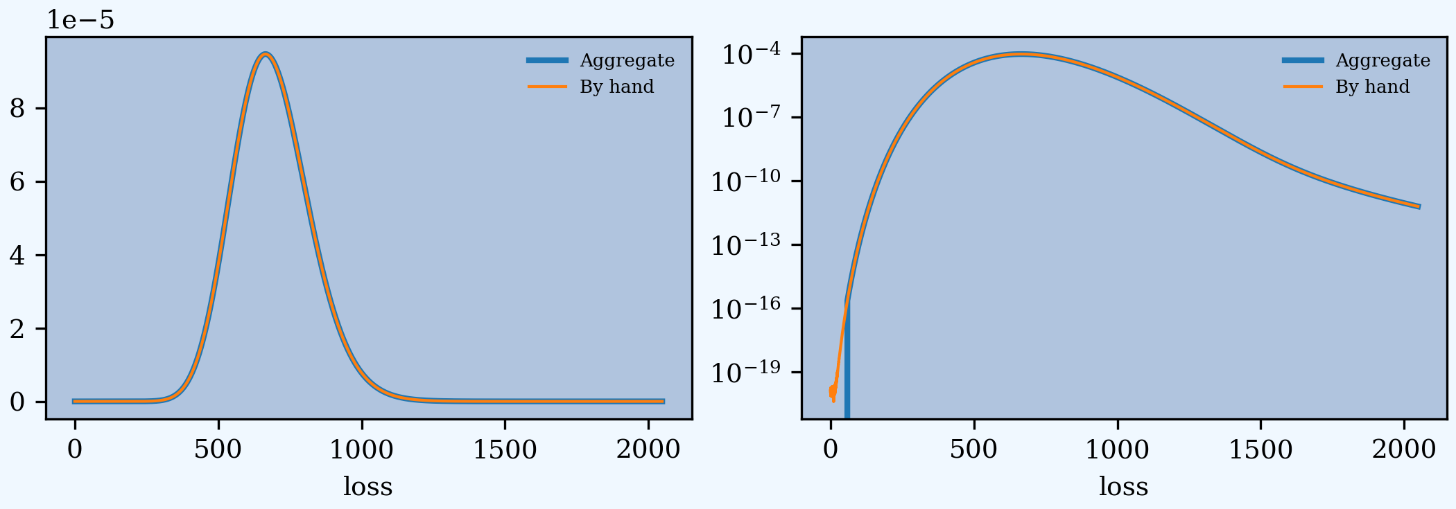
The very slight difference for small loss values arises because build removes numerical fuzz, setting values below machine epsilon (about 2e-16) to zero, explaining why the blue aggregate line drops off vertically on the left.
2.3.5.4. Basic Probability Functions
An Aggregate object acts like a discrete probability distribution. There are properties for the aggregate and severity mean, standard deviation, coefficient of variation, and skewness, both computed exactly and numerically estimated.
In [66]: print(a02.agg_m, a02.agg_sd, a02.agg_cv, a02.agg_skew)
50.0 31.622776601683793 0.6324555320336759 0.9486832980505139

In [67]: print(a02.est_m, a02.est_sd, a02.est_cv, a02.est_skew)
49.9999987284203 31.622777003581923 0.6324555561559914 0.9486832857144013

In [68]: print(a02.sev_m, a02.sev_sd, a02.sev_cv, a02.sev_skew)
10.0 10.0 1.0 2.0

In [69]: print(a02.est_sev_m, a02.est_sev_sd, a02.est_sev_cv, a02.est_sev_skew)
9.99999974568674 10.000000508623474 1.0000000762936754 1.9999996947979108
They have probability mass, cumulative distribution, survival, and quantile (inverse of distribution) functions.
In [70]: a02.pmf(60), a02.cdf(50), a02.sf(60), a02.q(a02.cdf(60)), a02.q(0.5)
Out[70]:
(np.float64(7.923645058165983e-05),
 np.float64(0.5639640504996987),
 np.float64(0.3244107518264777),
 np.float64(60.0),
 np.float64(44.90625))
The pdf, cdf, and sf for the underlying severity are also available.
In [71]: a02.sev.pdf(60), a02.sev.cdf(50), a02.sev.sf(60)
Out[71]:
(np.float64(0.00024787521766663585),
 np.float64(0.9932620530009145),
 np.float64(0.002478752176666357))
Note
Aggregate and Portfolio objects need to be updated after they have been created. Updating builds out discrete numerical approximations, analogous to simulation. By default, build() handles updating automatically.
Warning
Always use bucket sizes that have an exact binary representation (integers, 1/2, 1/4, 1/8, etc.) Never use 0.1 or 0.2 or other numbers that do not have an exact float representation, see REF.
2.3.5.5. Mixtures
An Aggregate can have a mixed severity. The mixture can include different distributions, parameters, shifts, and locations.
In [72]: a03 = build('agg TenM:03 '
   ....:             '25 claims '
   ....:             'sev [gamma lognorm invgamma] [5 10 10] cv [0.5 0.75 1.5] '
   ....:             '+ [0 10 20] wts [.5 .25 .25] '
   ....:             'mixed gamma 0.5'
   ....:            , bs=1/16)
   ....:

In [73]: qd(a03)

      E[X] Est E[X]    Err E[X]   CV(X) Est CV(X)  Skew(X) Est Skew(X)
X
Freq    25                      0.53852             1.0028
Sev     15   14.999 -3.7467e-05 0.90907   0.89065      inf      9.9075
Agg    375   374.99 -3.8034e-05 0.56838    0.5672      inf      1.0698
log2 = 16, bandwidth = 1/16, validation: fails sev cv, agg cv.
An Aggregate can model multiple units at once, and allow them to share mixing variables. This induces correlation between the components, see the report dataframe. All parts of the specification can vary, including limits and attachments (not shown). This case differentiated from a mixed severity by having no weights.
In [74]: a04 = build('agg TenM:04 '
   ....:             '[500 250 100] premium at [.8 .7 .5] lr '
   ....:             'sev [gamma lognorm invgamma] [5 10 10] cv [0.5 0.75 1.5] '
   ....:             'mixed gamma 0.5'
   ....:            , bs=1/8)
   ....:

In [75]: qd(a04)

       E[X] Est E[X]    Err E[X]   CV(X) Est CV(X)  Skew(X) Est Skew(X)
X
Freq  102.5                      0.50966             1.0002
Sev  6.0976   6.0975 -6.5732e-06 0.89437   0.87819      inf      43.583
Agg     625      625 -6.6355e-06 0.51726   0.51699      inf      1.0208
log2 = 16, bandwidth = 1/8, validation: fails sev cv.
2.3.5.6. Accessing Severity in an Aggregate
The attribute Aggregate.sevs is an array of the Severity
objects. Usually, it contains only one distribution but when severity is a
mixture it contains one for each mixture component. It can be iterated over.
Each Severity object wraps a scipy.stats continuous random
variable called fz that represents ground-up severity. The args are its
shape variable(s) and kwds its scale and location variables. This is
most interesting when the object has a mixed severity.
In [76]: for s in a03.sevs:
   ....:     print(s.sev_name, s.fz.args, s.fz.kwds)
   ....:
gamma (np.float64(4.0),) {'scale': np.float64(1.25), 'loc': np.float64(0.0)}
lognorm (np.float64(0.6680472308365776),) {'scale': np.float64(8.0), 'loc': np.float64(10.0)}
invgamma (np.float64(2.4444444444444446),) {'scale': np.float64(14.444444444444446), 'loc': np.float64(20.0)}
The property a03.sev is a namedtuple exposing the exact weighted pdf,
cdf, and sf of the underlying Severity objects.
In [77]: a03.sev.pdf(20), a03.sev.cdf(20), a03.sev.sf(20)
Out[77]:
(np.float64(0.014150102336136361),
 np.float64(0.657658211871339),
 np.float64(0.342341788128661))
The component weights are proportional to a03.en and a03.sev.cdf is computed as
In [78]: (np.array([s.cdf(20) for s in a03.sevs]) * a03.en).sum() / a03.en.sum()
Out[78]: np.float64(0.6576582118713391)
The following are equal using the defaut discretization method.
In [79]: a03.density_df.loc[20, 'F_sev'], a03.sev.cdf(20 + a03.bs/2)
Out[79]: (np.float64(0.658099359833043), np.float64(0.6580993598330431))
2.3.5.7. Reinsurance
Aggregate objects can apply per occurrence and aggregate reinsurance using clauses
occurrence net of [limit] xs ]attach]occurrence net of [pct] so [limit] xs [attach], wheresostands for “share of”occurrence ceded to [limit] xs ]attach]and so forth.
Examples.
Gross distribution: a triangular aggregate created as the sum of two uniform distribution on 1, 2,…, 10.
In [80]: a05g = build('agg TenM:05g dfreq [2] dsev [1:10]')

In [81]: qd(a05g)

      E[X] Est E[X]    Err E[X]   CV(X) Est CV(X) Skew(X) Est Skew(X)
X
Freq     2                            0
Sev    5.5      5.5           0 0.52223   0.52223       0           0
Agg     11       11 -3.3307e-16 0.36927   0.36927       0 -6.1064e-14
log2 = 6, bandwidth = 1, validation: not unreasonable.
Apply 3 xs 7 occurrence reinsurance to cap individual losses at 7. a05no is the net of occurrence distribution.
In [82]: a05no = build('agg TenM:05no dfreq [2] dsev [1:10] '
   ....:             'occurrence net of 3 xs 7')
   ....:

In [83]: qd(a05no)

      E[X] Est E[X] Err E[X]   CV(X) Est CV(X) Skew(X) Est Skew(X)
X
Freq     2                         0
Sev    5.5      4.9 -0.10909 0.52223   0.44197       0    -0.52103
Agg     11      9.8 -0.10909 0.36927   0.31252       0    -0.36842
log2 = 6, bandwidth = 1, validation: n/a, reinsurance.
Warning
The describe dataframe always reports gross analytic statistics (E[X], CV(X), Skew(X)) and the requested net or ceded estimated statistics (Est E[X], Est CV(X), Est Skew(X)). Look at the gross portfolio first to check computational accuracy. Net and ceded “error” report the difference to analytic gross.
Add an aggregate 4 xs 8 reinsurance cover on the net of occurrence distribution. a05n is the final net distribution.
In [84]: a05n = build('agg TenM:05n dfreq [2] dsev [1:10] '
   ....:            'occurrence net of 3 xs 7 '
   ....:            'aggregate net of 4 xs 8')
   ....:

In [85]: qd(a05n)

      E[X] Est E[X] Err E[X]   CV(X) Est CV(X) Skew(X) Est Skew(X)
X
Freq     2                         0
Sev    5.5      4.9 -0.10909 0.52223   0.44197       0    -0.52103
Agg     11     7.84 -0.28727 0.36927   0.20781       0     -1.2676
log2 = 6, bandwidth = 1, validation: n/a, reinsurance.
See The plot() Method for plots of the different distributions.
2.3.6. The Distortion Class
See Distortions and Spectral Risk Measures and PIR Chapter 10.5 for more information about distortions.
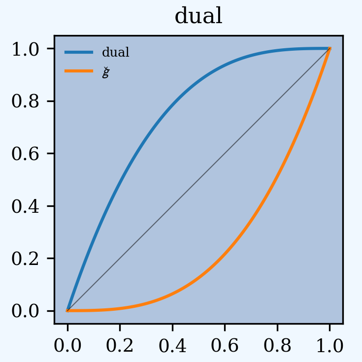
A Distortion can be created using DecL.
It object has methods for g, the distortion function, along with its dual g_dual(s)=1-g(1-s) and inverse g_inv. The plot() method shows g (above the diagonal) and g_inv (below).
In [86]: d06 = build('distortion TenM:06 dual 3')

In [87]: qd(d06.g(.2), d06.g_inv(.2), d06.g_dual(0.2),
   ....: d06.g(.8), d06.g_inv(.992), d06)
   ....:
0.488
0.071682
0.008
0.992
0.8
dual

In [88]: d06.plot();
The Distortion class can create distortions from a number of parametric families.
In [89]: from aggregate import Distortion

In [90]: Distortion.available_distortions(False, False)
Out[90]:
('ph',
 'wang',
 'cll',
 'lep',
 'ly',
 'clin',
 'dual',
 'ccoc',
 'tvar',
 'bitvar',
 'wtdtvar',
 'convex',
 'tt',
 'beta')
Run the command:
Distortion.test()
for graphs of samples from each available family. tt is not a distortion because it is not concave. It is included for historical reasons.
2.3.7. The Portfolio Class
A Portfolio object models a portfolio (book, block) of units (accounts, lines, business units, regions, profit centers), each represented as an Aggregate. It uses FFTs to convolve (add) the unit distributions. By default, all the units are assumed to be independent, though there are ways to adjust this. REF. The independence assumption is not as bad as it may appear; its effect can be ameliorated by selecting units carefully and sharing mixing variables appropriately (see REF for further discussion).
Portfolio objects have all of the attributes and methods of a Aggregate and add methods for pricing and allocation to units.
The DecL for a portfolio is simply:
port NAME AGG1 <AGG2> <AGG3> ...
where AGG1 is an aggregate specification. Portfolios can have one or more units. The DecL can be split over multiple lines if each aggregate begins on a new line and is indented by a tab (like a Python function).
Example.
Here is a three-unit portfolio built using a DecL program. The line breaks and horizontal spacing are cosmetic since Python just concatenates the input.
In [91]: p07 = build('port TenM:07 '
   ....:             'agg A '
   ....:                 '100 claims '
   ....:                 '10000 xs 0 '
   ....:                 'sev lognorm 100 cv 1.25 '
   ....:                 'poisson '
   ....:             'agg B '
   ....:                 '150 claims '
   ....:                 '2500 xs 5 '
   ....:                 'sev lognorm 50 cv 0.9 '
   ....:                 'mixed gamma .6 '
   ....:             'agg Cat '
   ....:                 '2 claims '
   ....:                 '1e5 xs 0 '
   ....:                 'sev 500 * pareto 1.8 - 500 '
   ....:                 'poisson'
   ....:            , approximation='exact', padding=2)
   ....:

In [92]: qd(p07)

             E[X] Est E[X]    Err E[X]   CV(X) Est CV(X)  Skew(X) Est Skew(X)
unit  X
A     Freq    100                          0.1                0.1
      Sev     100      100 -1.1973e-08  1.2498    1.2498   5.6619      5.6617
      Agg   10000    10000 -1.1973e-08 0.16006   0.16007   0.4082     0.40819
B     Freq    150                      0.60553             1.2001
      Sev  45.213   45.212 -1.2825e-05 0.99517   0.99528   3.4345      3.4335
      Agg  6781.9   6781.8 -1.2825e-05 0.61096   0.61096   1.2009      1.2009
Cat   Freq      2                      0.70711            0.70711
      Sev  616.02   616.02 -9.7399e-07  3.1331    3.1331   23.278      23.278
      Agg    1232     1232 -4.3508e-06  2.3256    2.3254   14.837      14.828
total Freq    252                      0.36266             1.1783
      Sev  71.484   71.483 -4.9016e-06  2.7998             172.51
      Agg   18014    18013 -2.6963e-05 0.29343   0.29322   2.9528       2.925
log2 = 16, bandwidth = 2, validation: not unreasonable.
The portfolio units are called A, B and Cat. Printing using qd shows p07.describe, which concatenates each unit’s describe and adds the same statistics for the total.
Unit A has 100 (expected) claims, each pulled from a lognormal distribution with mean of 30 and coefficient of variation 1.25 within the layer 100 xs 0 (i.e., losses are limited at 100). The frequency distribution is Poisson.
Unit B is similar.
The Cat unit is has expected frequency of 2 claims from the indicated limit, with severity given by a Pareto distribution with shape parameter 1.8, scale 500, shifted left by 500. This corresponds to the usual Pareto with survival function \(S(x) = (500 / (500 + x))^{1.8} = (1 + x / 500)^{-1.8}\) for \(x \ge 0\).
The portfolio total (i.e., the sum of the units) is computed using FFTs to convolve (add) the unit’s aggregate distributions. All computations use the same discretization bucket size; here the bucket-size bs=2. See For Portfolio Objects.
A Portfolio object acts like a discrete probability distribution, the same as an Aggregate. There are properties for the mean, standard deviation, coefficient of variation, and skewness, both computed exactly and numerically estimated.
In [93]: print(p07.agg_m, p07.agg_sd, p07.agg_cv, p07.agg_skew)
18013.930242377224 5285.799078302742 0.2934284194055587 2.952768695357267

In [94]: print(p07.est_m, p07.est_sd, p07.est_cv, p07.est_skew)
18013.444535982344 5281.917148506572 0.29322082947299716 2.924970410288626
They have probability mass, cumulative distribution, survival, and quantile (inverse of distribution) functions.
In [95]: p07.pmf(12000), p07.cdf(11000), p07.sf(12000), p07.q(p07.cdf(12000)), p07.q(0.5)
Out[95]:
(np.float64(9.808446441348987e-05),
 np.float64(0.031240713459622396),
 np.float64(0.9300376004823764),
 np.float64(12000.0),
 np.float64(17176.0))
The names of the units in a Portfolio are in a list called p07.unit_names or p07.unit_names_ex including total.
The Aggregate objects in the Portfolio can be iterated over.
In [96]: for u in p07:
   ....:     print(u.name, u.agg_m, u.est_m)
   ....:
A 9999.982520635807 9999.982400908266
B 6781.90965866976 6781.8226809277885
Cat 1232.038063071656 1232.0327026844775
2.3.8. Estimating Bucket Size for Discretization
Selecting an appropriate bucket size bs is critical to obtaining accurate results. This is a hard problem that may have hindered broad adoption of FFT-based methods.
See Numerical Methods and FFT Convolution for further discussion.
2.3.8.1. Hyper-parameters log2 and bs
The hyper-parameters log2 and bs control numerical calculations.
log2 equals the log to base 2 of the number of buckets used and bs
equals the bucket size. These values are printed by qd.
2.3.8.2. Estimating and Testing bs For Aggregate Objects
For an Aggregate, recommend_bucket() uses a shifted lognormal
method of moments fit and takes the recommend_p percentile as the
right-hand end of the discretization. By default recommend_p=0.999, but
for thick tailed distributions it may be necessary to use a value closer to
1. recommend_bucket() also considers any limits: ideally limits are
multiples of the bucket size.
The recommended value of bs should rounded up to a binary fraction
(denominator is a power of 2) using utilities.round_bucket().
Aggregate also includes two functions for assessing bs,
one based on the overall error and one based on looking at each severity
component.
Aggregate.aggregate_error_analysis() updates the object at a range of
different bs values and reports the total absolute (strictly, signed
absolute error) and relative error as well as an upper bound bs/2 on
the absolute value of the discretization error. log2 must be input and,
optionally, the log base 2 of the smallest bucket to model. It then models
six doublings of the input bucket. If no bucket is input, it models three
doublings up and down from the rounded recommend_bucket() suggestion.
The output table shows:
The actual
(agg, m)and estimated(est, m)means, from thedescribedataframe.The implied absolute
(abs, m)and relative(rel, m)errors in the mean.(rel, h)shows the maximum relative severity discretization error, which equalsbs / 2divided by the average severity.(rel, total), equal to the sum of(rel, h)andrel m.
Thick tailed distributions can favor a large bucket size without regard to the impact on discretization; accounting for the impact of bs / 2 is a countervailing force.
In [97]: qd(a04.aggregate_error_analysis(16), sparsify=False, col_space=9)

view            agg       est         abs         rel       rel        rel
stat              m         m           m           m         h      total
bs
0.03125         625    624.71    -0.28786 -0.00046057 0.0025625 -0.0030231
0.06250         625    624.99   -0.011699 -1.8718e-05  0.005125 -0.0051437
0.12500         625       625  -0.0041472 -6.6355e-06   0.01025  -0.010257
0.25000         625       625  -0.0015133 -2.4212e-06    0.0205  -0.020502
0.50000         625       625 -0.00050174 -8.0278e-07     0.041  -0.041001
1.00000         625       625   0.0026758  4.2813e-06     0.082   0.082004
2.00000         625    625.14     0.13828  0.00022125     0.164    0.16422
Aggregate.severity_error_analysis() performs a detailed error analysis of each severity component. It reports:
The name, limit, attachment, and truncation point for each severity component.
Sthe probability the component (or total losses) exceed the truncation.sum_pthe sum of discrete probabilities, which can be \(<1\) ifnormalize=False.wtthe weight of the component andenthe corresponding claim count.agg_meanandagg_wtthe aggregate mean contribution from the component (sums to the overall mean), and the each component’s proportion of the total. The loss weight can differ drastically from the count weight.meanandest_meanthe analytic and estimated severity by component and the correspondingabsandrelerror.trunc_errorthe truncation error by component (tail integral) and relative truncation error.The
h_errorbased onbs / 2by component, a (conservative) upper bound on discretization error and the relative error compared to the component mean.h2_adjandrel_h2_adjestimate a second order adjustment to the numerical mean. They give a better idea of the discretization error.
In [98]: qd(a04.severity_error_analysis(), line_width=75)

       name  limit  attachment  trunc          S  sum_p      wt    en  \
0     gamma    inf           0   8192          0      1 0.78049    80
1   lognorm    inf           0   8192 1.5989e-25      1 0.17073  17.5
2  invgamma    inf           0   8192 5.9297e-08      1 0.04878     5
3     total    inf           0   8192 8.6388e-08      1       1 102.5

   agg_mean  agg_wt   mean  est_mean         abs         rel  \
0       400    0.64      5         5  1.5997e-10  3.1994e-11
1       175    0.28     10        10 -1.6449e-12 -1.6449e-13
2        50    0.08     10    9.9992 -0.00082165 -8.2165e-05
3       625       1 6.0976    6.0975  -4.008e-05 -6.5732e-06

   trunc_error  rel_trunc_error  h_error  rel_h_error     h2_adj  \
0           -0               -0   0.0625       0.0125 5.1607e-09
1  -8.8373e-23      -8.8373e-24   0.0625      0.00625 1.0915e-14
2  -0.00033646      -3.3646e-05   0.0625      0.00625 1.1514e-14
3  -1.6408e-05      -2.6909e-06   0.0625      0.01025 4.0279e-09

   rel_h2_adj
0  1.0321e-09
1  1.0915e-15
2  1.1514e-15
3  6.6058e-10
Generally there is either discretization or truncation error. Look for one of them to dominate. Discretization error is solved with a smaller bucket; truncation with a larger. When the two conflict, add more buckets by increasing log2.
2.3.8.3. Estimating and Testing bs For Portfolio Objects
For a Portfolio, the right hand end of the distribution is estimated using the square root of sum of squares (proxy independent sum) of the right hand ends of each unit.
The method port.recommend_bucket() suggests a reasonable bucket size.
In [99]: print(p07.recommend_bucket().iloc[:, [0,3,6,10]])
             bs10       bs13      bs16      bs20
line
A       18.545709   2.318214  0.289777  0.018111
B       43.766975   5.470872  0.683859  0.042741
Cat    143.204295  17.900537  2.237567  0.139848
total  205.516978  25.689622  3.211203    0.2007

In [100]: p07.best_bucket(16)
Out[100]: 2
The column bsN corresponds to discretizing with 2**N buckets. The rows show suggested bucket sizes by unit and in total. For example with N=16 (i.e., 65,536 buckets) the suggestion is 2.19. It is best the bucket size is a divisor of any limits or attachment points. best_bucket() takes this into account and suggests 2.
To test bs, run the tests above on each unit.
2.3.9. Methods and Properties Common To Aggregate and Portfolio Classes
Aggregate and Portfolio both have the following methods and properties. See Aggregate Class and Portfolio Class for full lists.
infoanddescribeare dataframes with statistics and other information; they are printed with the object.density_dfa dataframe containing estimated probability distributions and other expected value information.The
statisticsdataframe shows analytically computed mean, variance, CV, and sknewness for each unit and in total.report_dfare dataframe with information to test if the numerical approximations appear valid. Numerically estimated statistics are prefacedest_orempirical.log2andbshyper-parameters that control numerical calculations.speca dictionary containing thekwargsneeded to recreate each object. For example, ifais anAggregateobject, thenAggregate(**a.spec)creates a new copy.spec_exa dictionary that appends hyper-parameters tospecincludinglog2andbs.programthe DecL program used to create the object. Blank if the object has been created directly. (A given object can often be created in different ways by DecL, so there is no obvious reverse mapping from thespec.)renamera dictionary used to rename columns of member dataframes to be more human readable.update()a method to run the numerical calculation of probability distributions.recommend_bucket()to recommend the value ofbs.Common statistical functions including pmf, cdf, sf, the quantile function (value at risk) and tail value at risk.
Statistical functions: pdf, cdf, sf, quantile, value at risk, tail value at risk, and so on.
plot()method to visualize the underlying distributions. Plots the pmf and log pmf functions and the quantile function. All the data is contained indensity_dfand the plots are created usingpandasstandard plotting commands.price()to apply a distortion (spectral) risk measure pricing rule with a variety of capital standards.snap()to round an input number to the index ofdensity_df.approximate()to create an analytic approximation.sample()pulls samples, see Samples from aggregate Object.
2.3.9.1. The info Dataframe
The info dataframe contains information about the frequency and severity stochastic models, how the object was computed, and any reinsurance applied (none in this case).
In [101]: print(a05n.info)
aggregate object name    TenM:05n
claim count              2.00
frequency distribution   empirical
severity distribution    dhistogram, unlimited.
bs                       1
log2                     6
padding                  1
sev_calc                 discrete
normalize                True
approximation            exact
validation_eps           0.0001
reinsurance              occurrence and aggregate
occurrence reinsurance   net of 100% share of 3 xs 7 per occurrence
aggregate reinsurance    net of 100% share of 4 xs 8 in the aggregate.
validation               n/a, reinsurance


In [102]: print(p07.info)
portfolio object name    TenM:07
aggregate objects        3
bs                       2
log2                     16
padding                  2
sev_calc                 discrete
normalize                True
last update              2026-05-18T14:27:53
hash                     3ca40f0204cf4b8b
2.3.9.2. The describe Dataframe
The describe dataframe contains gross analytic and estimated (net or ceded) statistics. When there is no reinsurance, comparison of analytic and estimated moments provides a test of computational accuracy (first case). It should always be reviewed after updating. When there is reinsurance, empirical is net (second case).
In [103]: qd(a05g.describe)

      E[X]  Est E[X]    Err E[X]   CV(X)  Est CV(X)  Err CV(X)  Skew(X)  Est Skew(X)
X
Freq     2       NaN         NaN       0        NaN        NaN      NaN          NaN
Sev    5.5       5.5           0 0.52223    0.52223          0        0            0
Agg     11        11 -3.3307e-16 0.36927    0.36927          0        0  -6.1064e-14

In [104]: with pd.option_context('display.max_columns', 15):
   .....:     print(a05n.describe)
   .....:
      E[X]  Est E[X]  Err E[X]     CV(X)  Est CV(X)  Err CV(X)  Skew(X)  Est Skew(X)
X
Freq   2.0       NaN       NaN  0.000000        NaN        NaN      NaN          NaN
Sev    5.5      4.90 -0.109091  0.522233   0.441968  -0.153697      0.0    -0.521027
Agg   11.0      7.84 -0.287273  0.369274   0.207810  -0.437247      0.0    -1.267573

In [105]: qd(p07.describe)

             E[X]  Est E[X]    Err E[X]   CV(X)  Est CV(X)   Err CV(X)  Skew(X)  Est Skew(X)
unit  X
A     Freq    100       NaN         NaN     0.1        NaN         NaN      0.1          NaN
      Sev     100       100 -1.1973e-08  1.2498     1.2498  1.0689e-05   5.6619       5.6617
      Agg   10000     10000 -1.1973e-08 0.16006    0.16007  6.5169e-06   0.4082      0.40819
B     Freq    150       NaN         NaN 0.60553        NaN         NaN   1.2001          NaN
      Sev  45.213    45.212 -1.2825e-05 0.99517    0.99528  0.00010815   3.4345       3.4335
      Agg  6781.9    6781.8 -1.2825e-05 0.61096    0.61096   1.913e-06   1.2009       1.2009
Cat   Freq      2       NaN         NaN 0.70711        NaN         NaN  0.70711          NaN
      Sev  616.02    616.02 -9.7399e-07  3.1331     3.1331   1.118e-06   23.278       23.278
      Agg    1232      1232 -4.3508e-06  2.3256     2.3254  -7.109e-05   14.837       14.828
total Freq    252       NaN         NaN 0.36266        NaN         NaN   1.1783          NaN
      Sev  71.484    71.483 -4.9016e-06  2.7998        NaN         NaN   172.51          NaN
      Agg   18014     18013 -2.6963e-05 0.29343    0.29322 -0.00070746   2.9528        2.925
Printing the object using qd add log2, bs, and validation information.
2.3.9.3. The density_df Dataframe
The density_df dataframe contains a wealth of information. It has 2**log2 rows and is indexed by the outcomes, all multiples of bs. Columns containing p are the probability mass function, of the aggregate or severity.
the aggregate and severity pmf (called
pand duplicated asp_totalfor consistency withPortfolioobjects), log pmf, cdf and sfthe aggregate lev (duplicated as
exa)exlea(less than or equal toa) which equals \(\mathsf E[X\mid X\le a]\) as a function oflossexgta(greater than) which equals \(\mathsf E[X\mid X > a]\)
In an Aggregate, p and p_total are identical, the latter included for consistency with Portfolio output. F and S are the cdf and sf (survival function). lev and exa are identical and equal the limited expected value at the loss level. Here are the first five rows.
In [106]: print(a05g.density_df.shape)
(64, 17)

In [107]: print(a05g.density_df.columns)
Index(['loss', 'p_total', 'p', 'p_sev', 'log_p', 'log_p_sev', 'F', 'F_sev', 'S', 'S_sev', 'lev', 'exa', 'exlea', 'e',
       'epd', 'exgta', 'exeqa'],
      dtype='object')

In [108]: with pd.option_context('display.max_columns', a05g.density_df.shape[1]):
   .....:     print(a05g.density_df.head())
   .....:
      loss  p_total     p  p_sev     log_p  log_p_sev     F  F_sev     S  S_sev   lev   exa     exlea     e       epd  \
loss
0.0    0.0     0.00  0.00    0.0      -inf       -inf  0.00    0.0  1.00    1.0  0.00  0.00       NaN  11.0  1.000000
1.0    1.0     0.00  0.00    0.1      -inf  -2.302585  0.00    0.1  1.00    0.9  1.00  1.00       NaN  11.0  0.909091
2.0    2.0     0.01  0.01    0.1 -4.605170  -2.302585  0.01    0.2  0.99    0.8  2.00  2.00  2.000000  11.0  0.818182
3.0    3.0     0.02  0.02    0.1 -3.912023  -2.302585  0.03    0.3  0.97    0.7  2.99  2.99  2.666667  11.0  0.728182
4.0    4.0     0.03  0.03    0.1 -3.506558  -2.302585  0.06    0.4  0.94    0.6  3.96  3.96  3.333333  11.0  0.640000

          exgta  exeqa
loss
0.0   11.000000    0.0
1.0   11.000000    1.0
2.0   11.090909    2.0
3.0   11.257732    3.0
4.0   11.489362    4.0
The Portfolio version is more exhaustive. It includes a variety of columns for each unit, suffixed _unit, and for the complement of each unit (sum of everything but that unit) suffixed _ημ_unit. The totals are suffixed _total. The most important columns are exeqa_unit, Conditional Expected Values. All the column names and a subset of density_df are shown next.
In [109]: print(p07.density_df.shape)
(65536, 46)

In [110]: print(p07.density_df.columns)
Index(['loss', 'p_A', 'p_B', 'p_Cat', 'p_total', 'F', 'S', 'exa_total', 'lev_total', 'exlea_total', 'e_total',
       'exgta_total', 'exeqa_total', 'exeqa_A', 'lev_A', 'exlea_A', 'e_A', 'exgta_A', 'exi_x_A', 'exi_xlea_A',
       'exi_xgta_A', 'exi_xeqa_A', 'exa_A', 'exeqa_B', 'lev_B', 'exlea_B', 'e_B', 'exgta_B', 'exi_x_B', 'exi_xlea_B',
       'exi_xgta_B', 'exi_xeqa_B', 'exa_B', 'exeqa_Cat', 'lev_Cat', 'exlea_Cat', 'e_Cat', 'exgta_Cat', 'exi_x_Cat',
       'exi_xlea_Cat', 'exi_xgta_Cat', 'exi_xeqa_Cat', 'exa_Cat', 'exi_xlea_sum', 'exi_xgta_sum', 'exi_xeqa_sum'],
      dtype='object')

In [111]: with pd.option_context('display.max_columns', p07.density_df.shape[1]):
   .....:     print(p07.density_df.filter(regex=r'[aipex012]_A').head())
   .....:
     p_A  exeqa_A  exlea_A          e_A      exgta_A   exi_x_A  exi_xlea_A  exi_xgta_A  exi_xeqa_A     exa_A
0.0  0.0      0.0      0.0  9999.982401  9999.982401  0.585913         0.0    0.585913         0.0  0.000000
2.0  0.0      0.0      0.0  9999.982401  9999.982401  0.585913         NaN    0.585913         0.0  1.171827
4.0  0.0      0.0      0.0  9999.982401  9999.982401  0.585913         NaN    0.585913         0.0  2.343653
6.0  0.0      0.0      0.0  9999.982401  9999.982401  0.585913         NaN    0.585913         0.0  3.515480
8.0  0.0      0.0      0.0  9999.982401  9999.982401  0.585913         NaN    0.585913         0.0  4.687306
2.3.9.4. The statistics Series and Dataframe
The statistics dataframe shows analytically computed mean, variance, CV, and sknewness. It is indexed by
severity name, limit and attachment,
freq1, freq2, freq3non-central frequency moments,sev1, sev2, sev3non-central severity moments, andthe mean, cv and skew(ness).
It applies to the gross outcome when there is reinsurance, so the results for a05g and a05no are the same.
In [112]: oco = ['display.width', 150, 'display.max_columns', 15,
   .....:         'display.float_format', lambda x: f'{x:.5g}']
   .....:

In [113]: with pd.option_context(*oco):
   .....:     print(a05g.statistics)
   .....:     print('\n')
   .....:     print(p07.statistics)
   .....:
name               TenM:05g
component  measure
limit                   inf
attachment             None
sevcv      param          0
el                       11
prem                      0
lr                        0
freq       ex1            2
           ex2            4
           ex3            8
           mean           2
           cv             0
           skew         NaN
sev        ex1          5.5
           ex2         38.5
           ex3        302.5
           mean         5.5
           cv       0.52223
           skew           0
agg        ex1           11
           ex2        137.5
           ex3       1875.5
           mean          11
           cv       0.36927
           skew           0
mix        cv         [2.0]
wt                        1


                           A          B        Cat      total
component measure
freq      ex1            100        150          2        252
          ex2          10100      30750          6      71856
          ex3     1.0301e+06 7.9868e+06         22 2.3216e+07
          mean           100        150          2        252
          cv             0.1    0.60553    0.70711    0.36266
          skew           0.1     1.2001    0.70711     1.1783
sev       ex1            100     45.213     616.02     71.484
          ex2          25621     4068.7 4.1047e+06      45166
          ex3      1.674e+07 6.7987e+05 1.7449e+11 1.3919e+09
          mean           100     45.213     616.02     71.484
          cv          1.2498    0.99517     3.1331     2.7998
          skew        5.6619     3.4345     23.278     172.51
agg       ex1          10000     6781.9       1232      18014
          ex2     1.0256e+08 6.3163e+07 9.7273e+06 3.5244e+08
          ex3     1.0785e+12 7.4665e+11 3.8119e+11 7.7915e+12
          mean         10000     6781.9       1232      18014
          cv         0.16006    0.61096     2.3256    0.29343
          skew        0.4082     1.2009     14.837     2.9528
          limit        10000       2500      1e+05      1e+05
          P99.9e       15944      27628      41971      56972
2.3.9.5. The report_df Dataframe
The report_df dataframe combines information from statistics with
estimated moments to test if the numerical approximations appear valid. It
is an expanded version of describe. Numerically estimated statistics are
prefaced est or empirical.
In [114]: with pd.option_context(*oco):
   .....:     print(a05g.report_df)
   .....:     print('\n')
   .....:     print(p07.report_df)
   .....:
view               0 independent     mixed   empirical       error
statistic
name        TenM:05g    TenM:05g  TenM:05g
limit            inf         inf       inf
attachment                     0         0
el                11          11        11
freq_m             2           2         2
freq_cv            0           0         0
freq_skew
sev_m            5.5         5.5       5.5         5.5           0
sev_cv       0.52223     0.52223   0.52223     0.52223           0
sev_skew           0           0         0           0
agg_m             11          11        11          11 -3.3307e-16
agg_cv       0.36927     0.36927   0.36927     0.36927           0
agg_skew           0           0         0 -6.1064e-14        -inf


unit                   A           B         Cat       total
statistic
freq_m               100         150           2         252
freq_cv              0.1     0.60553     0.70711     0.36266
freq_skew            0.1      1.2001     0.70711      1.1783
sev_m                100      45.213      616.02      71.484
sev_cv            1.2498     0.99517      3.1331      2.7998
sev_skew          5.6619      3.4345      23.278      172.51
agg_m              10000      6781.9        1232       18014
agg_emp_m          10000      6781.8        1232       18013
agg_m_err    -1.1973e-08 -1.2825e-05 -2.7692e-05 -2.6963e-05
agg_cv           0.16006     0.61096      2.3256     0.29343
agg_emp_cv       0.16007     0.61096      2.3249     0.29322
agg_cv_err    6.5168e-06  1.9129e-06 -0.00027305 -0.00070746
agg_skew          0.4082      1.2009      14.837      2.9528
agg_emp_skew     0.40819      1.2009      14.818       2.925
agg_skew_err -1.3542e-05  1.6688e-08  -0.0012766  -0.0094143
agg_emp_kurt     0.40604      2.1621      381.65      33.187
P99.0_emp          14206       19834       10246       33586
P99.6_emp          14956       22626       16610       38304
The report_df provides extra information when there is a mixed severity.
In [115]: with pd.option_context(*oco):
   .....:     print(a03.report_df)
   .....:
view              0        1        2 independent    mixed empirical       error
statistic
name        TenM:03  TenM:03  TenM:03     TenM:03  TenM:03
limit           inf      inf      inf         inf      inf
attachment                                      0        0
el             62.5      125    187.5         375      375
freq_m         12.5     6.25     6.25          25       25
freq_cv     0.57446  0.64031  0.64031     0.36572  0.53852
freq_skew    1.0097   1.0307   1.0307     0.66199   1.0028
sev_m             5       20       30          15       15    14.999 -3.7467e-05
sev_cv          0.5    0.375  0.50002     0.90907  0.90907   0.89065   -0.020261
sev_skew          1   2.6716      inf         inf      inf    9.9075          -1
agg_m          62.5      125    187.5         375      375    374.99 -3.8034e-05
agg_cv      0.59161  0.65765  0.67082     0.41265  0.56838    0.5672  -0.0020722
agg_skew     1.0238   1.0613      inf         inf      inf    1.0698          -1
The dataframe shows statistics for each mixture component, columns 0,1,2,
their sum if they are added independently and their sum if there is a shared
mixing variable, as there is here. The common mixing induces correlation
between the mix components, acting to increases the CV and skewness, often
dramatically.
2.3.9.6. The spec and spec_ex Dictionaries
The spec dictionary contains the input information needed to create each
object. For example, if a is an Aggregate, then Aggregate
(**a.spec) creates a new copy. spec_ex appends meta-information to
spec about hyper-parameters.
In [116]: from pprint import pprint

In [117]: pprint(a05n.spec)
{'agg_kind': 'net of',
 'agg_reins': [(1.0, 4.0, 8.0)],
 'exp_attachment': None,
 'exp_el': 0,
 'exp_en': -1,
 'exp_limit': inf,
 'exp_lr': 0,
 'exp_premium': 0,
 'freq_a': array([2.]),
 'freq_b': array([1.]),
 'freq_name': 'empirical',
 'freq_p0': nan,
 'freq_zm': False,
 'name': 'TenM:05n',
 'note': '',
 'occ_kind': 'net of',
 'occ_reins': [(1.0, 3.0, 7.0)],
 'sev_a': nan,
 'sev_b': 0,
 'sev_conditional': True,
 'sev_cv': 0,
 'sev_lb': 0,
 'sev_loc': 0,
 'sev_mean': 0,
 'sev_name': 'dhistogram',
 'sev_pick_attachments': None,
 'sev_pick_losses': None,
 'sev_ps': array([0.1, 0.1, 0.1, 0.1, 0.1, 0.1, 0.1, 0.1, 0.1, 0.1]),
 'sev_scale': 0,
 'sev_ub': inf,
 'sev_wt': 1,
 'sev_xs': array([ 1.,  2.,  3.,  4.,  5.,  6.,  7.,  8.,  9., 10.])}
2.3.9.7. The DecL Program
The program property returns the DecL program used to create the object.
It is blank if the object was not created using DecL. The helper function pprint_ex() pretty prints a program.
In [118]: from aggregate import pprint_ex

In [119]: pprint_ex(a05n.program, split=20)
agg TenM:05n
  dfreq [2]
  dsev [1:10]
  occurrence net of 3 xs 7
  aggregate net of 4 xs 8
Out[119]: 'agg TenM:05n\n  dfreq [2]\n  dsev [1:10]\n  occurrence net of 3 xs 7\n  aggregate net of 4 xs 8'

In [120]: pprint_ex(p07.program, split=20)
port TenM:07
  agg A
    100 claims 10000 xs 0
    sev lognorm 100 cv 1.25
    poisson
  agg B
    150 claims 2500 xs 5
    sev lognorm 50 cv 0.9
    mixed gamma .6
  agg Cat
    2 claims 1e5 xs 0
    sev 500 * pareto 1.8 - 500
    poisson
Out[120]: 'port TenM:07\n  agg A\n    100 claims 10000 xs 0\n    sev lognorm 100 cv 1.25\n    poisson\n  agg B\n    150 claims 2500 xs 5\n    sev lognorm 50 cv 0.9\n    mixed gamma .6\n  agg Cat\n    2 claims 1e5 xs 0\n    sev 500 * pareto 1.8 - 500\n    poisson'
2.3.9.8. The update() Method
After an Aggregate or a Portfolio object has been created it needs to be updated to populate its density_df dataframe. build() automatically updates the objects it creates with default hyper-parameter values. Sometimes it is necessary to re-update with different hyper-parameters. The update() method takes arguments log2=13, bs=0, and recommend_p=0.999. The first two control the number and size of buckets. When bs==0 it is estimated using the method recommend_bucket(). If bs!=0 then recommend_p is ignored.
Further control over updating is available, as described in REF.
2.3.9.9. Statistical Functions
Aggregate and Portfolio objects include basic mean, CV, standard deviation, variance, and skewness statistics as attributes. Those prefixed agg are based on exact calculations:
agg_m,agg_cv,agg_sd,agg_var, andagg_skew
and prefixed est are based on the estimated numerical statistics:
est_m,est_cv,est_sd,est_var, andest_skew.
In addition, Aggregate has similar series prefixed sev and
est_sev for the exact and estimated numerical severity. These attributes
are just conveniences; they are all available in (or derivable from)
report_df.
Aggregate and Portfolio objects act like scipy.stats (continuous) frozen random variable objects and include the following statistical functions.
pmf()the probability mass functionpdf()the probability density function—broadly interpreted—defined as the pmf divided bybscdf()the cumulative distribution functionsf()the survival functionq()the quantile function (left inverse cdf), also known as value at risktvar()tail value at risk functionvar_dict()a dictionary of tail statistics by unit and in total
We aren’t picky about whether the density is technically a density when the aggregate is actually mixed or discrete.
The discrete output (density_df.p_*) is interpreted as the distribution, so none of the statistical functions is interpolated.
For example:
In [121]: qd(a05g.pmf(2), a05g.pmf(2.2), a05g.pmf(3), a05g.cdf(2), a05g.cdf(2.2))
0.01
0
0.02
0.01
0.01

In [122]: print(1 - a05g.cdf(2), a05g.sf(2))
0.99 0.99

In [123]: print(a05g.q(a05g.cdf(2)))
2.0
The last line illustrates that q() and cdf() are inverses. The var_dict() function computes tail statistics for all units, return in a dictionary.
In [124]: p07.var_dict(0.99), p07.var_dict(0.99, kind='tvar')
Out[124]:
({'A': np.float64(14206.0),
  'B': np.float64(19834.0),
  'Cat': np.float64(10246.0),
  'total': np.float64(33586.0)},
 {'A': np.float64(15025.781065020969),
  'B': np.float64(22845.877658808236),
  'Cat': np.float64(20360.451246691864),
  'total': np.float64(41763.10848598601)})
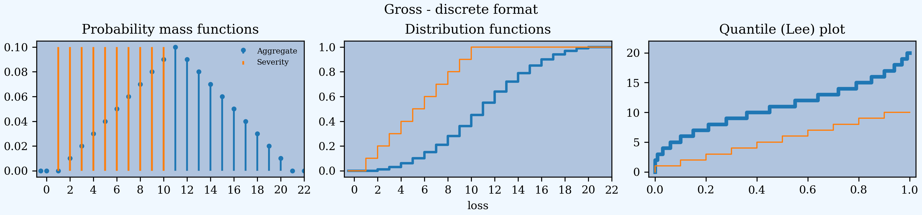
2.3.9.10. The plot() Method
The plot() method provides basic visualization. There are three plots: the pdf/pmf for severity and the aggregate on the left. The middle plot shows log density for continuous distributions and the distribution function for discrete ones (selected when bs==1 and the mean is < 100). The right plot shows the quantile (or VaR or Lee) plot.
The reinsurance examples below show the discrete output format. The plots show the
gross, net of occurrence, and net severity and aggregate pmf (left) and cdf
(middle), and the quantile (Lee) plot (right). The property a05g.figure
returns the last figure made by the object as a convenience. You could also
use plt.gcf().
In [125]: a05g.plot()
In [126]: a05g.figure.suptitle('Gross - discrete format');
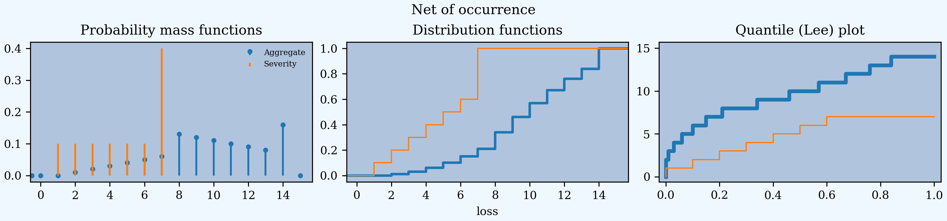
In [127]: a05no.plot()
In [128]: a05no.figure.suptitle('Net of occurrence');
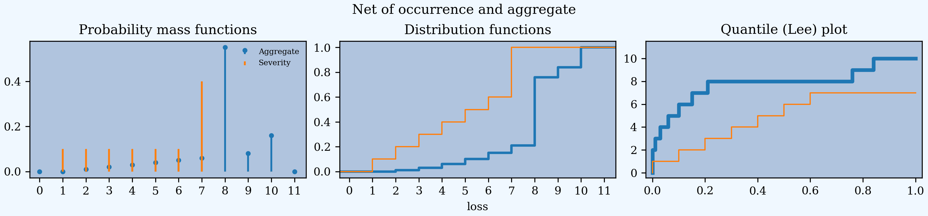
In [129]: a05n.plot()
In [130]: a05n.figure.suptitle('Net of occurrence and aggregate');
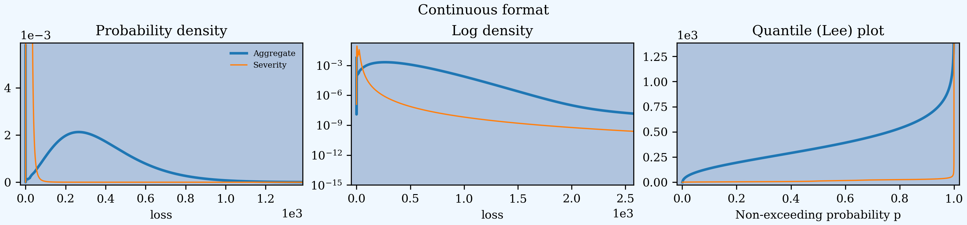
Continuous distributions substitute the log density for the distribution in the middle.
In [131]: a03.plot()

In [132]: a03.figure.suptitle('Continuous format');
A Portfolio object plots the density and log density of each unit and
the total.
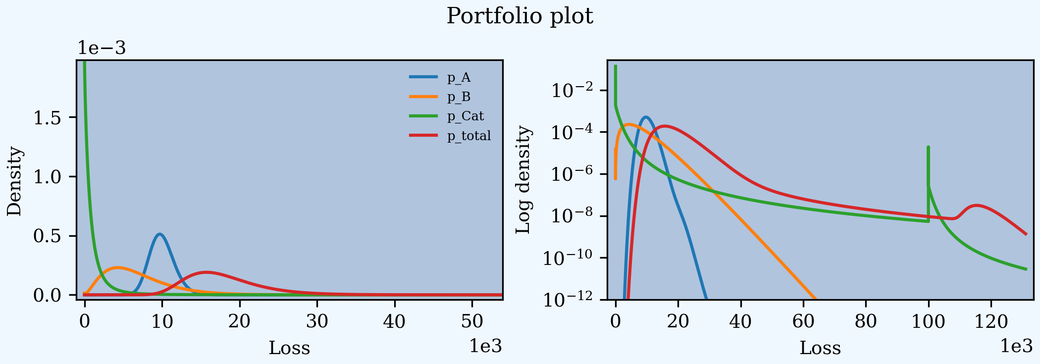
In [133]: p07.plot()

In [134]: p07.figure.suptitle('Portfolio plot');
2.3.9.11. The price() Method
The price() method computes the risk adjusted expected value (technical price net of expenses) of losses limited by capital at a specified VaR threshold. Suppose the 99.9%ile outcome is used to specify regulatory assets \(a\).
In [135]: qd(a03.q(0.999))
1358
The risk adjustment is specified by a spectral risk measure corresponding to an input distortion. Distortions can be built using DecL, see The Distortion Class. price() applies to \(X\wedge a\).
It returns expected limited losses L, the risk adjusted premium P, the margin M = P - L, the capital Q = a - P, the loss ratio, leverage as premium to capital PQ, and return on capital ROE.
In [136]: qd(a03.price(0.999, d06).T)

line       TenM:03
statistic
L           374.82
P           558.25
M           183.43
Q           799.75
a             1358
LR         0.67142
PQ         0.69802
ROE        0.22936
When price() is applied to a Portfolio, it returns the total premium and its (lifted) natural allocation to each unit, see PIR Chapter 14, along with all the other statistics in a dataframe. Losses are allocated by equal priority in default.
In [137]: qd(p07.price(0.999, d06).df.T)

distortion     dual
unit              A       B      Cat   total
statistic
L            9997.3  6779.8   1212.4   17990
P             10448  9874.5   1913.8   22236
M            450.25  3094.7   701.35  4246.2
Q            7656.6   10203    12817   30662
a             18104   20078    14731   52898
LR           0.9569 0.68659  0.63352 0.80904
PQ           1.3645 0.96781  0.14932 0.72519
COC        0.058806 0.30332 0.054721 0.13848
The ROE varies by unit, reflecting different consumption and cost of capital by layer. The less risky unit A runs at a higher loss ratio (cheaper insurance) but higher ROE than unit B because it consumes more expensive, equity-like lower layer capital but less capital overall (higher leverage).
2.3.9.12. The snap() Method
snap() rounds an input number to the index of density_df. It selects the nearest element.
2.3.9.13. The approximate() Method
The approximate() method creates an analytic approximation fit using moment matching. Normal, lognormal, gamma, shifted lognormal, and shifted gamma distributions can be fit, the last two requiring three moments. To fit all five and return a dictionary call with argument "all".
In [138]: fzs = a03.approximate('all')

In [139]: d = pd.DataFrame({k: fz.stats('mvs') for k, fz in fzs.items()},
   .....:          index=pd.Index(['mean', 'var', 'skew'], name='stat'),
   .....:                 dtype=float)
   .....:

In [140]: qd(d)

       norm  gamma  lognorm  sgamma  slognorm
stat
mean 374.99 374.99   374.99  374.99    374.99
var   45238  45238    45238   45238     45238
skew      0 1.1344   1.8841  1.0698    1.0698
2.3.10. Additional Portfolio Methods
2.3.10.1. Conditional Expected Values
A Portfolio object’s density_df includes a slew of values to allocate capital (please don’t) or margin (please do). These all rely on what Mildenhall and Major [2022] call the \(\kappa\) function, defined for a sum \(X=\sum_i X_i\) as the conditional expectation
Notice that \(\sum_i \kappa_i(x)=x\), hinting at its allocation application.
See PIR Chapter 14.3 for an explanation of why \(\kappa\) is so useful. In short, it shows which units contribute to bad overall outcomes. It is in density_df as the columns exeqa_unit, read as the “expected value given X eq(uals) a”.
Here are some \(\kappa\) values and graph for p07. Looking the log density plot on the right shows that unit B dominates for moderately large events, but Cat dominates for the largest events.
In [141]: fig, axs = plt.subplots(1, 2, figsize=(2 * 3.5, 2.45)); \
   .....: ax0, ax1 = axs.flat; \
   .....: lm = [-1000, 65000]; \
   .....: bit = p07.density_df.filter(regex='exeqa_[ABCt]').rename(
   .....:     columns=lambda x: x.replace('exeqa_', '')).sort_index(axis=1); \
   .....: bit.index.name = 'Loss'; \
   .....: bit.plot(xlim=lm, ylim=lm, ax=ax0); \
   .....: ax0.set(title=r'$E[X_i\mid X]$', aspect='equal'); \
   .....: ax0.axhline(bit['B'].max(), lw=.5, c='C7');
   .....:

In [142]: p07.density_df.filter(regex='p_[ABCt]').rename(
   .....:     columns=lambda x: x.replace('p_', '')).plot(ax=ax1, xlim=lm, logy=True);
   .....:

In [143]: ax1.set(title='Log density');

In [144]: bit['Pct A'] = bit['A'] / bit.index

In [145]: qd(bit.loc[:lm[1]:1024])

             A      B    Cat  total   Pct A
Loss
0.0          0      0      0      0     NaN
2048.0       0      0      0   2048       0
4096.0  3729.8 307.48 58.741   4096 0.91059
6144.0  5419.3 602.16 122.54   6144 0.88205
8192.0  6911.6 1062.4 217.99   8192  0.8437
10240.0 8133.9 1757.5 348.62  10240 0.79432
12288.0 9041.7 2735.6 510.69  12288 0.73582
14336.0 9655.4 3986.6 694.09  14336  0.6735
16384.0  10048 5445.7 890.17  16384 0.61329
18432.0  10299 7035.3   1098  18432 0.55874
20480.0  10464 8692.1 1324.3  20480 0.51092
22528.0  10576  10370 1582.2  22528 0.46946
...        ...    ...    ...    ...     ...
40960.0  10622  17734  12604  40960 0.25932
43008.0  10551  16531  15926  43008 0.24532
45056.0  10477  15060  19519  45056 0.23253
47104.0  10408  13547  23149  47104 0.22096
49152.0  10349  12178  26625  49152 0.21055
51200.0  10301  11051  29847  51200 0.20119
53248.0  10264  10185  32799  53248 0.19276
55296.0  10236 9545.6  35515  55296 0.18511
57344.0  10214 9085.2  38045  57344 0.17812
59392.0  10197 8755.1  40440  59392 0.17169
61440.0  10184   8516  42740  61440 0.16575
63488.0  10172 8339.2  44976  63488 0.16023

The thin horizontal line at the maximum value of exeqa_B (left plot) shows that \(\kappa_B\) is not increasing. Unit B contributes more to moderately bad outcomes than Cat, but in the tail Cat dominates.
Using filter(regex=...) to select columns from density_df is a helpful idiom. The total column is labeled _total. Using upper case for unit names makes them easier to select.
2.3.10.2. Calibrate Distortions
The calibrate_distortions() method calibrates distortions to achieve requested pricing for the total loss. Pricing can be requested by loss ratio or return on capital (ROE). Asset levels can be specified in monetary terms, or as a probability of non-exceedance. To calibrate the usual suspects (constant cost of capital, proportional hazard, dual, Wang, and TVaR) to achieve a 15% return with a 99.6% capital level run:
In [146]: p07.calibrate_distortions(Ps=[0.996], ROEs=[0.15], strict='ordered');

In [147]: qd(p07.distortion_df)

                                S     L     P     PQ     Q  COC   param  std_param      error
a       LR       method
38304.0 0.871293 ccoc   0.0039991 17962 20615 1.1654 17689 0.15    0.15    0.13043          0
                 ph     0.0039991 17962 20615 1.1654 17689 0.15 0.61919    0.23518  1.095e-09
                 wang   0.0039991 17962 20615 1.1654 17689 0.15 0.51526     0.2844 4.7105e-06
                 dual   0.0039991 17962 20615 1.1654 17689 0.15  2.0031    0.33402 -2.794e-09
                 tvar   0.0039991 17962 20615 1.1654 17689 0.15 0.37271    0.37271 9.7863e-06

In [148]: pprint(p07.dists)
{'ccoc': ccoc, 'dual': dual, 'ph': ph, 'tvar': tvar, 'wang': wang}
The answer is returned in the dist_ans dataframe. The requested distortions are all single parameter, returned in the param column. The last column gives the error in achieved premium. The attribute p07.dists is a dictionary with keys distortion types and values Distortion objects. See PIR REF for more discussion.
2.3.10.3. Analyze Distortions
The analyze_distortions() method applies the distortions in p07.dists at a given capital level and summarizes the implied (lifted) natural allocations across units. Optionally, it applies a number of traditional (bullshit) pricing methods. The answer dataframe includes premium, margin, expected loss, return, loss ratio and leverage statistics for each unit and method. Here is a snippet, again at the 99.6% capital level.
In [149]: ans = p07.analyze_distortions(p=0.996)

In [150]: print(ans.comp_df.xs('LR', axis=0, level=1).
   .....:      to_string(float_format=lambda x: f'{x:.1%}'))
   .....:
line            A      B   Cat  total
Method
Dist ccoc  109.8% 103.8% 24.0%  87.1%
Dist dual   96.9%  77.8% 75.4%  87.1%
Dist ph     99.0%  80.6% 56.4%  87.1%
Dist tvar   96.3%  77.8% 77.8%  87.1%
Dist wang   97.7%  78.6% 67.7%  87.1%
EL          87.1%  87.1% 87.1%  87.1%
EPD         96.0%  78.3% 10.3%  58.6%
EqRiskEPD   99.7%  90.7% 38.4%  87.1%
EqRiskTVaR  95.7%  83.5% 58.0%  87.1%
EqRiskVaR   95.5%  82.7% 61.0%  87.1%
MerPer      97.9%  88.9% 66.0%  91.5%
ScaledEPD  107.9%  99.5% 26.3%  87.1%
ScaledTVaR  99.0%  85.3% 46.3%  87.1%
ScaledVaR   99.3%  84.9% 46.5%  87.1%
TVaR        94.3%  78.0% 38.0%  80.1%
VaR         93.9%  76.6% 37.3%  79.2%
coTVaR      99.1%  83.5% 49.3%  87.1%
covar       97.6%  80.6% 60.5%  87.1%
2.3.10.4. Twelve Plot
The twelve_plot() method produces a detailed analysis of the behavior of a two unit portfolio. To run it, build the portfolio and calibrate some distortions. Then apply one of the distortions (to compute an augmented version of density_df with pricing information). We give two examples.
First, the case of a thin-tailed and a thick-tailed unit. Here, the thick tailed line benefits from pooling at low capital levels, resulting in negative margins to the thin-tail line in compensation. At moderate to high capital levels the total margin for both lines is positive. Assets are 12.5. The argument efficient=False in apply_distortion() includes extra columns in density_df that are needed to compute the plot.
In [151]: p09 = build('port TenM:09 '
   .....:               'agg X1 1 claim sev gamma 1 cv 0.25 fixed '
   .....:               'agg X2 1 claim sev 0.7 * lognorm 1 cv 1.25 + 0.3 fixed'
   .....:              , bs=1/1024)
   .....:

In [152]: qd(p09)

            E[X] Est E[X]    Err E[X]   CV(X) Est CV(X) Skew(X) Est Skew(X)
unit  X
X1    Freq     1                            0
      Sev      1        1 -5.5511e-16    0.25      0.25     0.5         0.5
      Agg      1        1 -5.5511e-16    0.25      0.25     0.5         0.5
X2    Freq     1                            0
      Sev      1  0.99999 -1.0796e-05   0.875   0.87452  5.7031       5.603
      Agg      1  0.99999 -1.0796e-05   0.875   0.87452  5.7031       5.603
total Freq     2                            0
      Sev      1  0.99999  -5.398e-06 0.64348            7.1845
      Agg      2        2 -5.8107e-06 0.45501   0.45476  5.0802      4.9869
log2 = 16, bandwidth = 1/1024, validation: fails sev skew, agg skew.

In [153]: print(f'Asset P value {p09.cdf(12.5):.5g}')
Asset P value 0.99958

In [154]: p09.calibrate_distortions(ROEs=[0.1], As=[12.5], strict='ordered');

In [155]: qd(p09.distortion_df)

                              S      L      P      PQ      Q  COC   param  std_param       error
a    LR       method
12.5 0.676722 ccoc   0.00041558 1.9985 2.9531 0.30933 9.5469  0.1     0.1   0.090909           0
              ph     0.00041558 1.9985 2.9531 0.30933 9.5469  0.1 0.51152    0.32317   1.998e-08
              wang   0.00041558 1.9985 2.9531 0.30933 9.5469  0.1 0.88394    0.46806  1.6577e-06
              dual   0.00041558 1.9985 2.9531 0.30933 9.5469  0.1  4.4902    0.63572 -2.0466e-10
              tvar   0.00041558 1.9985 2.9531 0.30933 9.5469  0.1 0.71207    0.71207  6.2397e-06

In [156]: p09.apply_distortion('dual', efficient=False);

In [157]: fig, axs = plt.subplots(4, 3, figsize=(3 * 3.5, 4 * 2.45), constrained_layout=True)

In [158]: p09.twelve_plot(fig, axs, p=0.999, p2=0.999)
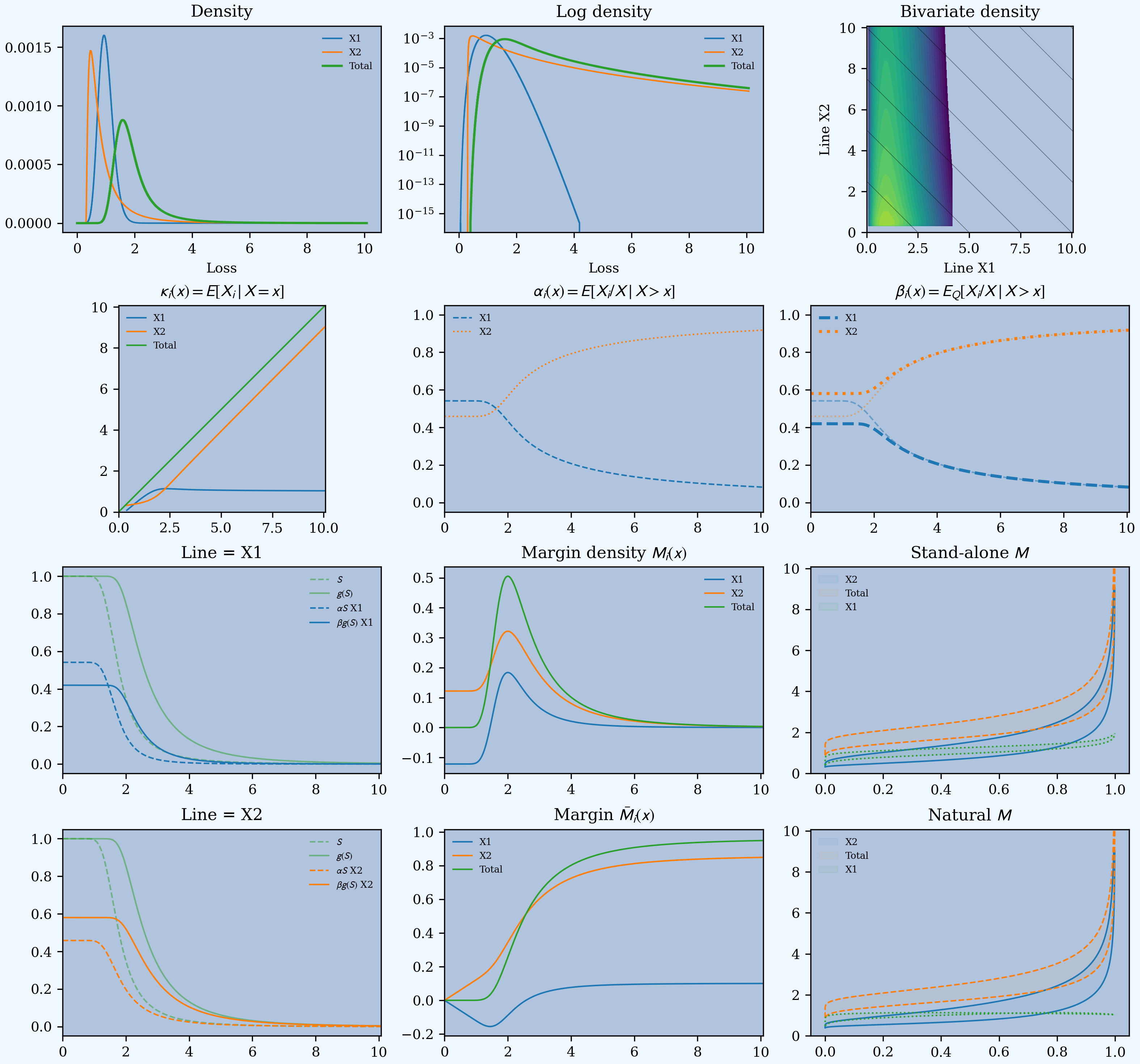
There is a lot of information here. We refer to the charts as \((r,c)\) for row \(r=1,2,3,4\) and column \(c=1,2,3\), starting at the top left. The horizontal axis shows the asset level in all charts except \((3,3)\) and \((4,3)\), where it shows probability, and \((1,3)\) where it shows loss. Blue represents the thin tailed unit, orange thick tailed and green total. When both dashed and solid lines appear on the same plot, the solid represent risk-adjusted and dashed represent non-risk-adjusted functions. Here is the key.
\((1,1)\) shows density for \(X_1, X_2\) and \(X=X_1+X_2\); the two units are independent. Both units have mean 1.
\((1,2)\): log density; comparing tail thickness.
\((1,3)\): the bivariate log-density. This plot illustrates where \((X_1, X_2)\) lives. The diagonal lines show \(X=k\) for different \(k\). These show that large values of \(X\) correspond to large values of \(X_2\), with \(X_1\) about average.
\((2,1)\): the form of \(\kappa_i\) is clear from looking at \((1,3)\). \(\kappa_1\) peaks above 1.0 around \(x=2\) and hereafter it declines to 1.0. \(\kappa_2\) is monotonically increasing.
\((2,2)\): The \(\alpha_i\) functions. For small \(x\) the expected proportion of losses is approximately 50/50, since the means are equal. As \(x\) increases \(X_2\) dominates. The two functions sum to 1.
\((2,3)\): The thicker lines are \(\beta_i\) and the thinner lines \(\alpha_i\) from \((2,2)\). Since \(\alpha_1\) decreases \(\beta_1(x)\le \alpha_1(x)\). This can lead to \(X_1\) having a negative margin in low asset layers. \(X_2\) is the opposite.
\((3,1)\): illustrates premium and margin determination by asset layer for \(X_1\). For low asset layers \(\alpha_1(x) S(x)>\beta_1(x) g(S(x))\) (dashed above solid) corresponding to a negative margin. Beyond about \(x=1.38\) the lines cross and the margin is positive.
\((4,1)\): shows the same thing for \(X_2\). Since \(\alpha_2\) is increasing, \(\beta_2(x)>\alpha_2(x)\) for all \(x\) and so all layers get a positive margin. The solid line \(\beta_2 gS\) is above the dashed \(\alpha_2 S\) line.
\((3,2)\): the layer margin densities. For low asset layers premium is fully funded by loss with zero overall margin. \(X_2\) requires a positive margin and \(X_1\) a negative one, reflecting the benefit the thick unit receives from pooling in low layers. The overall margin is always non-negative. Beyond about \(x=1.5\), \(X_1\)’s margin is also positive.
\((4,2)\): the cumulative margin in premium by asset level. Total margin is zero in low dollar-swapping layers and then increases. It is always non-negative. The curves in this plot are the integrals of those in \((3,2)\) from 0 to \(x\).
\((3,3)\): shows stand-alone loss \((1-S(x),x)=(p,q(p))\) (dashed) and premium \((1-g(S(x)),x)=(p,q(1-g^{-1}(1-p))\) (solid, shifted left) for each unit and total. The margin is the shaded area between the two. Each set of three lines (solid or dashed) does not add up vertically because of diversification. The same distortion \(g\) is applied to each unit to the stand-alone \(S_{X_i}\). It is calibrated to produce a 10 percent return overall. On a stand-alone basis, calculating capital by unit to the same return period as total, \(X_1\) is priced to a 77.7 percent loss ratio and \(X_2\) 52.5 percent, producing an average 62.7 percent, vs. 67.6 percent on a combined basis. Returns are 37.5 percent and 9.4 percent respectively, averaging 11.5 percent, vs 10 percent on a combined basis, see stand-alone analysis below.
\((4,3)\): shows the natural allocation of loss and premium to each unit. The total (green) is the same as \((3,3)\). For each \(i\), dashed shows \((p, \mathsf E[X_i\mid X=q(p)])\), i.e. the expected loss recovery conditioned on total losses \(X=q(p)\), and solid shows \((p, \mathsf E[X_i\mid X=q(1-g^{-1}(1-p))])\), i.e. the natural premium allocation. Here the solid and dashed lines add up vertically: they are allocations of the total. Looking vertically above \(p\), the shaded areas show how the total margin at that loss level is allocated between lines. \(X_1\) mostly consumes assets at low layers, and the blue area is thicker for small \(p\), corresponding to smaller total losses. For \(p\) close to 1, large total losses, margin is dominated by \(X_2\) and in fact \(X_1\) gets a slight credit (dashed above solid). The change in shape of the shaded margin area for \(X_1\) is particularly evident: it shows \(X_1\) benefits from pooling and requires a lower overall margin.
There may appear to be a contradiction between figures \((3,2)\) and \((4,3)\) but it should be noted that a particular \(p\) value in \((4,3)\) refers to different events on the dotted and solid lines.
Plots \((3,3)\) and \((4,3)\) explain why the thick unit requires relatively more margin: its shape does not change when it is pooled with \(X_1\). In \((3,3)\) the green shaded area is essentially an upwards shift of the orange, and the orange areas in \((3,3)\) and \((3,4)\) are essentially the same. This means that adding \(X_1\) has virtually no impact on the shape of \(X_2\); it is like adding a constant. This can also be seen in \((4,3)\) where the blue region is almost a straight line.
Applying the same distortion on a stand-alone basis produces:
In [159]: a = p09.stand_alone_pricing(p09.dists['dual'], p=p09.cdf(12.5))

In [160]: print(a.iloc[:8])
line                X1         X2        sop      total
method  stat
sa dual L     0.999956   0.998459   1.998414   1.998459
        LR    0.777176   0.525226   0.626922   0.676722
        M     0.286697   0.902547   1.189244   0.954686
        P     1.286652   1.901006   3.187658   2.953145
        PQ    1.681666   0.198284   0.307915   0.309332
        Q     0.765106   9.587275  10.352381   9.546855
        ROE   0.374715   0.094140   0.114876   0.100000
        a     2.051758  11.488281  13.540039  12.500000
The lifted natural allocation (diversified pricing) is given next. These numbers are so different than the stand-alone because X2 has to compensate X1 for the transfer of wealth in default states. When there is a large loss, it is caused by X2 and so X2 receives a disproportionate share of the assets in default.
In [161]: a2 = p09.analyze_distortion('dual', ROE=0.1, p=p09.cdf(12.5))

In [162]: print(a2.pricing.unstack(1).droplevel(0, axis=0).T)
line             X1        X2     total
     stat
12.5 L     0.999920  0.998539  1.998459
     LR    0.908669  0.538958  0.676722
     M     0.100502  0.854183  0.954686
     P     1.100422  1.852722  2.953145
     PQ    0.888570  0.222992  0.309332
     Q     1.238419  8.308458  9.546855
     ROE   0.081154  0.102809  0.100000
The second portfolio has been selected with two thick tailed units. A appears riskier at lower return periods and B at higher. Pricing is calibrated to a 15% ROE at a 99.6% capital level.
In [163]: p10 = build('port TenM:10 '
   .....:              'agg A '
   .....:                  '30 claims '
   .....:                  '1000 xs 0 '
   .....:                  'sev gamma 25 cv 1.5 '
   .....:                  'mixed delaporte 0.75 0.6 '
   .....:              'agg B '
   .....:                  '5 claims '
   .....:                  '20000 xs 20 '
   .....:                  'sev lognorm 25 cv 3.0 '
   .....:                  'poisson'
   .....:             , bs=1)
   .....:

In [164]: qd(p10)

             E[X] Est E[X]    Err E[X]   CV(X) Est CV(X)  Skew(X) Est Skew(X)
unit  X
A     Freq     30                       0.7719             3.5645
      Sev      25   24.989 -0.00045632     1.5     1.501        3      2.9984
      Agg     750   749.66 -0.00045632 0.81904   0.81911   3.2482      3.2478
B     Freq      5                      0.44721            0.44721
      Sev  55.582    55.58 -3.0222e-05  2.3472    2.3473   18.671      18.671
      Agg  277.91    277.9 -3.0222e-05   1.141     1.141   6.9737      6.9737
total Freq     35                      0.66471             3.5156
      Sev  29.369   29.359 -0.00034112  2.0855             27.142
      Agg  1027.9   1027.6 -0.00034112 0.67253   0.67256   2.9521      2.9519
log2 = 16, bandwidth = 1, validation: fails sev mean, agg mean.

In [165]: p10.calibrate_distortions(ROEs=[0.15], Ps=[0.996], strict='ordered');

In [166]: qd(p10.distortion_df)

                              S      L      P      PQ      Q  COC   param  std_param      error
a      LR      method
4596.0 0.68709 ccoc   0.0039969 1023.3 1489.3 0.47937 3106.7 0.15    0.15    0.13043          0
               ph     0.0039969 1023.3 1489.3 0.47937 3106.7 0.15 0.57953     0.2662 3.9482e-06
               wang   0.0039969 1023.3 1489.3 0.47937 3106.7 0.15 0.64115    0.34971  3.716e-06
               dual   0.0039969 1023.3 1489.3 0.47937 3106.7 0.15  2.6459    0.45143 2.2737e-13
               tvar   0.0039969 1023.3 1489.3 0.47937 3106.7 0.15 0.52695    0.52695 8.0193e-06
Apply the dual distortion and then create the twelve plot.
In [167]: p10.apply_distortion('dual', efficient=False);

In [168]: fig, axs = plt.subplots(4, 3, figsize=(3 * 3.5, 4 * 2.45), constrained_layout=True)

In [169]: p10.twelve_plot(fig, axs, p=0.999995, p2=0.999999)

Applying the same distortion on a stand-alone basis produces:
In [170]: assets = p10.q(0.996)

In [171]: a = p10.stand_alone_pricing(p10.dists['dual'], p=p10.cdf(assets))

In [172]: print(a.iloc[:8])
line                    A            B          sop        total
method  stat
sa dual L      745.845783   274.056275  1019.902058  1023.266475
        LR       0.652332     0.590524     0.634487     0.687090
        M      397.506631   190.033998   587.540629   466.008721
        P     1143.352413   464.090274  1607.442687  1489.275195
        PQ       0.383850     0.309206     0.358840     0.479371
        Q     2978.647587  1500.909726  4479.557313  3106.724805
        ROE      0.133452     0.126613     0.131160     0.150000
        a     4122.000000  1965.000000  6087.000000  4596.000000
The lifted natural allocation (diversified pricing) is given next.
In [173]: a2 = p10.analyze_distortion('dual', ROE=0.1, p=p10.cdf(assets))

In [174]: print(a2.pricing.unstack(1).droplevel(0, axis=0).T)
line                   A           B        total
       stat
4596.0 L      746.454112  276.812363  1023.266475
       LR       0.752826    0.776418     0.759066
       M      245.081324   79.712633   324.793957
       P      991.535436  356.524996  1348.060432
       PQ       0.379589    0.560741     0.415051
       Q     2612.128741  635.810828  3247.939568
       ROE      0.093824    0.125372     0.100000
2.3.11. Extensions
The extensions sub-package contains additional classes and functions that are either peripheral to the main project or still under development (and subject to change). Currently, extensions includes:
case_studiesfor creating and managing PIR case studies (see Case Studies).pir_figuresfor creating various exhibits and figures in PIR.figuresfor creating various other exhibits and figures.samplesincludes functions for working with samples and executing a switcheroo. Eventually, these will be integrated intoPortfolio.
2.3.12. Summary of Objects Created by DecL
Each of the objects created by build() is automatically stored in the knowledge. We can list them out now.
In [175]: from aggregate import pprint_ex

In [176]: for n, r in build.qlist('^TenM:').iterrows():
   .....:     pprint_ex(r.program, split=20)
   .....:
agg TenM:01
  100 claims 100 xs 0
  sev lognorm 10 cv 1.25
  poisson
agg TenM:02
  5 claims
  sev gamma 10 cv 1
  poisson
agg TenM:03
  25 claims
  sev [gamma lognorm invgamma] [5 10 10] cv [0.5 0.75 1.5] + [0 10 20]
  wts [.5 .25 .25]
  mixed gamma 0.5
agg TenM:04 [500 250 100] premium at [.8 .7 .5] lr
  sev [gamma lognorm invgamma] [5 10 10] cv [0.5 0.75 1.5]
  mixed gamma 0.5
agg TenM:05g
  dfreq [2]
  dsev [1:10]
agg TenM:05n
  dfreq [2]
  dsev [1:10]
  occurrence net of 3 xs 7
  aggregate net of 4 xs 8
agg TenM:05no
  dfreq [2]
  dsev [1:10]
  occurrence net of 3 xs 7
distortion TenM:06 dual 3
port TenM:07
  agg A
    100 claims 10000 xs 0
    sev lognorm 100 cv 1.25
    poisson
  agg B
    150 claims 2500 xs 5
    sev lognorm 50 cv 0.9
    mixed gamma .6
  agg Cat
    2 claims 1e5 xs 0
    sev 500 * pareto 1.8 - 500
    poisson
port TenM:09
  agg X1
    1 claim
    sev gamma 1 cv 0.25
    fixed
  agg X2
    1 claim
    sev 0.7 * lognorm 1 cv 1.25 + 0.3
    fixed
port TenM:10
  agg A
    30 claims 1000 xs 0
    sev gamma 25 cv 1.5
    mixed delaporte 0.75 0.6
  agg B
    5 claims 20000 xs 20
    sev lognorm 25 cv 3.0
    poisson
sev TenM:Gamma gamma 10 cv .5
sev TenM:Invgamma invgamma 10 cv .5
sev TenM:Invgauss invgauss 10 cv .5
sev TenM:Lognorm lognorm 10 cv .5
sev TenM:Sev.1 lognorm 80 cv .5
sev TenM:Sev.2 10 * lognorm 1 cv .5 + 70
agg TenM:SevLayer
  1 claim 15 xs 5
  sev gamma 10 cv .5
  fixed