2.5. Individual Risk Pricing
Objectives: Applications of the Aggregate class to individual risk pricing, including LEVs, ILFs, layering, and the insurance charge and savings (Table L, M), illustrated using problems from CAS Part 8.
Audience: Individual risk large account pricing, broker, or risk retention actuary.
Prerequisites: DecL, underwriting and insurance terminology, aggregate distributions, risk measures.
See also: Reinsurance Pricing, The Reinsurance Clauses. For other related examples see Published Problems and Examples, especially Bahnemann Monograph. Self-Insurance Plan Stop-Loss Insurance for theoretical background.
Contents:
The examples in this section are illustrative. aggregate gives the gross,
ceded, and net distributions and with those in hand, it is possible to answer
any reasonable question about a large account program.
2.5.1. Helpful References
2.5.2. Insurance Charge and Insurance Savings in Aggregate
Creating a custom table of insurance charges and savings, varying with account
size, specific occurrence limit, and entry ratio (aggregate limit) is very
easy using aggregate. We will make a custom function to illustrate one
solution.
First, we need a severity curve. This step is very important, and would be
customized to the state and hazard group distribution of expected losses. We
use a simple mixture of a lognormal for small claims and a Pareto for large
claims, with a mean of about 25 (work in 000s). Create it as an object in the
knowledge using build(). The parameters are selected judgmentally.
In [1]: from aggregate import build, qd

In [2]: mu, sigma, shape, scale, wt = \
   ...:     -0.204573975,  1.409431871, 1.633490596, 57.96737143, 0.742942461
   ...:

In [3]: mean = wt * np.exp(mu + sigma**2 / 2) + (1 - wt) * scale / (shape - 1)

In [4]: build(f'sev IR:WC '
   ...:       f'[exp({mu}) {scale}] * [lognorm pareto] [{sigma} {shape}] '
   ...:       f'+ [0 {-scale}] wts [{wt} {1-wt}]');
   ...:

In [5]: print(f'Mean = {mean:.1f} in 000s')
Mean = 25.2 in 000s
Second, we will build the model for a large account with 350 expected claims and an occurrence limit of 100M. This model is used to set the update parameters. Assume a gamma mixed Poisson frequency distribution with a mixing CV of 25% throughout. The CV could be an input parameter in a production application.
In [6]: a01 = build('agg IR:Base '
   ...:             '350 claims '
   ...:             '100000 xs 0 '
   ...:             'sev sev.IR:WC '
   ...:             'mixed gamma 0.25 ',
   ...:             update=False)
   ...:

In [7]: qd(a01)

       E[X]   CV(X)  Skew(X)
X
Freq    350 0.25565  0.50012
Sev  24.947  10.172   177.37
Agg  8731.6  0.6008   7.3319
log2 = 0, bandwidth = na, validation: n/a, not updated.

In [8]: qd(a01.statistics.loc['sev', [0, 1, 'mixed']])

name         0          1      mixed
measure
ex1     2.2005      90.69     24.947
ex2     35.299 2.5281e+05      65013
ex3     4127.8 1.1293e+10 2.9029e+09
mean    2.2005      90.69     24.947
cv       2.508     5.4532     10.172
skew    23.299     92.803     177.37
Look at the aggregate_error_analysis to pick bs (see Estimating and Testing bs For Aggregate Objects). Use an expanded number of buckets log2=19 because the mixture
includes small mean lognormal and large mean Pareto components (some trial
and error not shown).
In [9]: err_anal = a01.aggregate_error_analysis(19)

In [10]: qd(err_anal, sparsify=False)

view      agg    est     abs         rel       rel        rel
stat        m      m       m           m         h      total
bs
0.0625 8731.6 8552.1 -179.54   -0.020562 0.0012526  -0.021815
0.1250 8731.6 8647.1 -84.529  -0.0096808 0.0025053  -0.012186
0.2500 8731.6 8731.1 -0.5447 -6.2382e-05 0.0050105 -0.0050729
0.5000 8731.6 8728.8  -2.798 -0.00032045  0.010021  -0.010342
1.0000 8731.6 8719.9 -11.715  -0.0013417  0.020042  -0.021384
2.0000 8731.6 8694.4 -37.172  -0.0042572  0.040084  -0.044341
4.0000 8731.6 8639.2 -92.465    -0.01059  0.080168  -0.090758
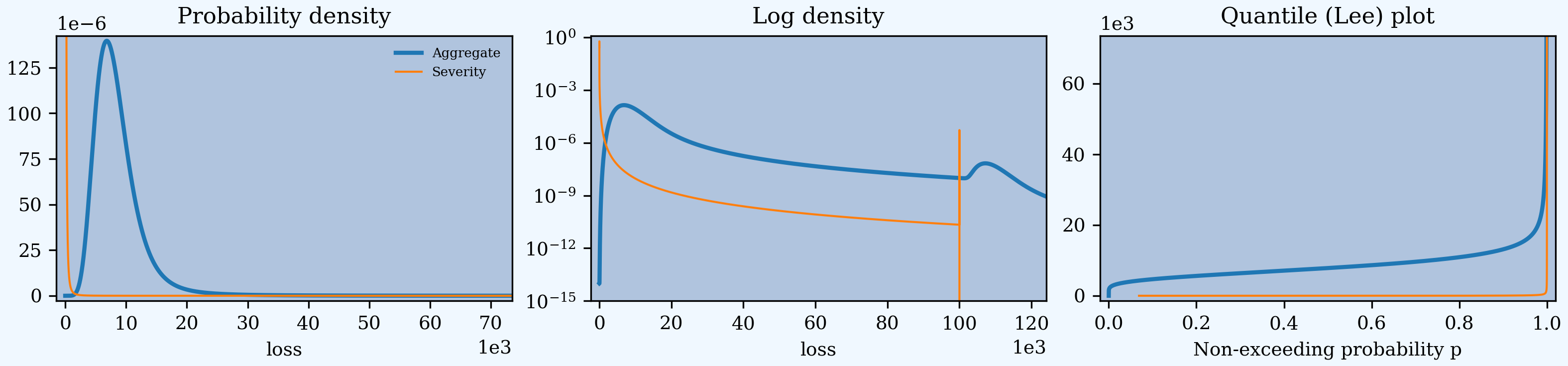
Select bs=1/4 as the most accurate from the displayed range (``
(‘rel’, ‘m’)``). Update and plot. The plot shows the impact of the occurrence
limit in the extreme right tail.
In [11]: a01.update(approximation='exact', log2=19, bs=1/4, normalize=False)

In [12]: qd(a01)

       E[X] Est E[X]    Err E[X]   CV(X) Est CV(X)  Skew(X) Est Skew(X)
X
Freq    350                      0.25565            0.50012
Sev  24.947   24.946 -5.5033e-05  10.172    10.172   177.37      177.37
Agg  8731.6   8731.1 -6.2382e-05  0.6008   0.60063   7.3319      7.3121
log2 = 19, bandwidth = 1/4, validation: not unreasonable.

In [13]: a01.plot()
Third, create a custom function of account size and the occurrence limit, to
produce the Aggregate object and a small table of insurance savings
and charges. Account size is measured by the expected ground-up claim count.
It should be clear how to extend this function to include custom severity,
different mixing CVs, or produce factors for different entry ratios. The
answer is returned in a namedtuple.
In [14]: from collections import namedtuple

In [15]: def make_table(claims=360, occ_limit=100000):
   ....:     """
   ....:     Make a table of insurance charges and savings by entry ratio for
   ....:     specified account size (expected claim count) and specific
   ....:     occurrence limit.
   ....:     """
   ....:     a01 = build(f'agg IR:{claims}:{occ_limit} '
   ....:                 f'{claims} claims '
   ....:                 f'{occ_limit} xs 0 '
   ....:                  'sev sev.IR:WC '
   ....:                  'mixed gamma 0.25 '
   ....:                 , approximation='exact', log2=19, bs=1/4, normalize=False)
   ....:     er_table = np.linspace(.1, 2., 20)
   ....:     df = a01.density_df
   ....:     ix = df.index.get_indexer(er_table * a01.est_m, method='nearest')
   ....:     df = a01.density_df.iloc[ix][['loss', 'F', 'S', 'e', 'lev']]
   ....:     df['er'] = er_table
   ....:     df['charge'] = (df.e - df.lev) / a01.est_m
   ....:     df['savings'] = (df.loss - df.lev) / a01.est_m
   ....:     df['entry'] = df.loss / a01.est_m
   ....:     df = df.set_index('entry')
   ....:     df = df.drop(columns=['e',  'er'])
   ....:     df.index = [f"{x:.2f}" for x in df.index]
   ....:     df.index.name = 'r'
   ....:     Table = namedtuple('Table', ['ob', 'table_df'])
   ....:     return Table(a01, df)
   ....:
Finally, apply the new function to create some tables.
A small account with 25 expected claims, about 621K limited losses, and a low 50K occurrence limit. The output shows the usual
describediagnostics for the underlyingAggregateobject, followed by a small Table across different entry ratios. The Table is indexed by entry ratio(aggregate attachment as a proportion of limited losses) and showslossthe aggregate limit loss level in currency units; the cdf and sf at that loss level (the latter giving the probability the aggregate layer attaches); the limited expected value at the entry ratiolev; and the insurance charge(1 - lev / loss) and savings (r - lev / loss).
In [16]: tl = make_table(25, 50)

In [17]: fc = lambda x: f'{x:,.1f}' if abs(x) > 10 else f'{x:.3f}'

In [18]: qd(tl.ob)

       E[X] Est E[X]    Err E[X]   CV(X) Est CV(X)  Skew(X) Est Skew(X)
X
Freq     25                      0.32016            0.51537
Sev  9.2527   9.2513 -0.00014797  1.7107     1.711   1.8407      1.8405
Agg  231.32   231.28 -0.00014797 0.46857   0.46862  0.65759     0.65759
log2 = 19, bandwidth = 1/4, validation: fails sev mean, agg mean.

In [19]: qd(tl.table_df, float_format=fc, col_space=8)

             loss        F        S      lev   charge  savings
r
0.10         23.2    0.005    0.995     23.2    0.900    0.000
0.20         46.2    0.017    0.983     46.0    0.801    0.001
0.30         69.5    0.041    0.959     68.6    0.703    0.004
0.40         92.5    0.081    0.919     90.2    0.610    0.010
0.50        115.8    0.135    0.865    111.0    0.520    0.021
0.60        138.8    0.205    0.795    130.1    0.438    0.037
0.70        162.0    0.284    0.716    147.7    0.361    0.062
0.80        185.0    0.370    0.630    163.2    0.294    0.094
0.90        208.2    0.459    0.541    176.8    0.236    0.136
1.00        231.2    0.544    0.456    188.3    0.186    0.186
1.10        254.5    0.625    0.375    197.9    0.144    0.245
1.20        277.5    0.696    0.304    205.7    0.110    0.310
1.30        300.8    0.760    0.240    212.0    0.083    0.384
1.40        323.8    0.813    0.187    216.9    0.062    0.462
1.50        347.0    0.857    0.143    220.8    0.045    0.546
1.60        370.0    0.892    0.108    223.7    0.033    0.633
1.70        393.2    0.920    0.080    225.8    0.024    0.724
1.80        416.2    0.941    0.059    227.4    0.017    0.816
1.90        439.5    0.958    0.042    228.6    0.012    0.912
2.00        462.5    0.970    0.030    229.4    0.008    1.008
The impact of increasing the occurrence limit to 250K:
In [20]: tl2 = make_table(25, 250)

In [21]: qd(tl2.ob)

       E[X] Est E[X]    Err E[X]   CV(X) Est CV(X)  Skew(X) Est Skew(X)
X
Freq     25                      0.32016            0.51537
Sev  16.989   16.988 -8.0799e-05  2.5894    2.5897    3.852       3.852
Agg  424.73   424.69 -8.0799e-05 0.60885   0.60889  0.91444     0.91445
log2 = 19, bandwidth = 1/4, validation: not unreasonable.

In [22]: qd(tl2.table_df, float_format=fc, col_space=8)

             loss        F        S      lev   charge  savings
r
0.10         42.5    0.015    0.985     42.3    0.900    0.001
0.20         85.0    0.052    0.948     83.4    0.804    0.004
0.30        127.5    0.104    0.896    122.7    0.711    0.011
0.40        170.0    0.164    0.836    159.5    0.624    0.025
0.50        212.2    0.227    0.773    193.5    0.544    0.044
0.60        254.8    0.291    0.709    225.0    0.470    0.070
0.70        297.2    0.358    0.642    253.7    0.403    0.102
0.80        339.8    0.428    0.572    279.6    0.342    0.142
0.90        382.2    0.497    0.503    302.4    0.288    0.188
1.00        424.8    0.562    0.438    322.4    0.241    0.241
1.10        467.2    0.622    0.378    339.7    0.200    0.300
1.20        509.8    0.677    0.323    354.6    0.165    0.365
1.30        552.0    0.726    0.274    367.2    0.135    0.435
1.40        594.5    0.770    0.230    377.9    0.110    0.510
1.50        637.0    0.808    0.192    386.9    0.089    0.589
1.60        679.5    0.842    0.158    394.3    0.072    0.672
1.70        722.0    0.870    0.130    400.4    0.057    0.757
1.80        764.5    0.894    0.106    405.4    0.046    0.846
1.90        807.0    0.915    0.085    409.4    0.036    0.936
2.00        849.5    0.931    0.069    412.7    0.028    1.029
The impact of increasing the account size to 250 expected claims, still at 250K occurrence limit:
In [23]: tl3 = make_table(250, 250)

In [24]: qd(tl3.ob)

       E[X] Est E[X]    Err E[X]   CV(X) Est CV(X)  Skew(X) Est Skew(X)
X
Freq    250                      0.25788            0.50024
Sev  16.989   16.988 -8.0799e-05  2.5894    2.5897    3.852       3.852
Agg  4247.3   4246.9 -8.0799e-05 0.30548   0.30549  0.52614     0.52615
log2 = 19, bandwidth = 1/4, validation: not unreasonable.

In [25]: qd(tl3.table_df, float_format=fc, col_space=8)

             loss        F        S      lev   charge  savings
r
0.10        424.8    0.000    1.000    424.7    0.900    0.000
0.20        849.5    0.000    1.000    849.5    0.800    0.000
0.30      1,274.0    0.001    0.999  1,273.7    0.700    0.000
0.40      1,698.8    0.009    0.991  1,696.7    0.600    0.000
0.50      2,123.5    0.031    0.969  2,113.8    0.502    0.002
0.60      2,548.2    0.080    0.920  2,516.2    0.408    0.008
0.70      2,972.8    0.161    0.839  2,890.8    0.319    0.019
0.80      3,397.5    0.272    0.728  3,224.5    0.241    0.041
0.90      3,822.2    0.402    0.598  3,506.5    0.174    0.074
1.00      4,247.0    0.535    0.465  3,732.1    0.121    0.121
1.10      4,671.8    0.657    0.343  3,903.0    0.081    0.181
1.20      5,096.2    0.760    0.240  4,025.9    0.052    0.252
1.30      5,521.0    0.840    0.160  4,110.1    0.032    0.332
1.40      5,945.8    0.898    0.102  4,165.1    0.019    0.419
1.50      6,370.5    0.937    0.063  4,199.6    0.011    0.511
1.60      6,795.0    0.963    0.037  4,220.4    0.006    0.606
1.70      7,219.8    0.979    0.021  4,232.5    0.003    0.703
1.80      7,644.5    0.988    0.012  4,239.3    0.002    0.802
1.90      8,069.2    0.994    0.006  4,243.0    0.001    0.901
2.00      8,494.0    0.997    0.003  4,244.9    0.000    1.000
Finally, increase the occurrence limit to 10M:
In [26]: tl4 = make_table(250, 10000)

In [27]: qd(tl4.ob)

       E[X] Est E[X]    Err E[X]   CV(X) Est CV(X)  Skew(X) Est Skew(X)
X
Freq    250                      0.25788            0.50024
Sev   24.26   24.258 -5.6594e-05  6.2915    6.2918   33.759      33.759
Agg  6064.9   6064.6 -5.6594e-05 0.47416   0.47418   1.6385      1.6386
log2 = 19, bandwidth = 1/4, validation: not unreasonable.

In [28]: qd(tl4.table_df, float_format=fc, col_space=8)

             loss        F        S      lev   charge  savings
r
0.10        606.5    0.000    1.000    606.5    0.900    0.000
0.20      1,213.0    0.001    0.999  1,212.9    0.800    0.000
0.30      1,819.2    0.008    0.992  1,817.1    0.700    0.000
0.40      2,425.8    0.033    0.967  2,412.5    0.602    0.002
0.50      3,032.2    0.086    0.914  2,984.7    0.508    0.008
0.60      3,638.8    0.168    0.832  3,515.7    0.420    0.020
0.70      4,245.2    0.272    0.728  3,989.4    0.342    0.042
0.80      4,851.8    0.385    0.615  4,396.7    0.275    0.075
0.90      5,458.0    0.496    0.504  4,735.5    0.219    0.119
1.00      6,064.5    0.595    0.405  5,010.4    0.174    0.174
1.10      6,671.0    0.680    0.320  5,229.3    0.138    0.238
1.20      7,277.5    0.750    0.250  5,401.4    0.109    0.309
1.30      7,884.0    0.805    0.195  5,535.8    0.087    0.387
1.40      8,490.5    0.847    0.153  5,640.8    0.070    0.470
1.50      9,096.8    0.880    0.120  5,723.1    0.056    0.556
1.60      9,703.2    0.905    0.095  5,788.1    0.046    0.646
1.70     10,309.8    0.924    0.076  5,839.8    0.037    0.737
1.80     10,916.2    0.938    0.062  5,881.6    0.030    0.830
1.90     11,522.8    0.949    0.051  5,915.7    0.025    0.925
2.00     12,129.0    0.958    0.042  5,943.8    0.020    1.020
These Tables all behave as expected. The insurance charge decreases with increasing expected losses (claim count) and decreasing occurrence limit.
2.5.3. Summary of Objects Created by DecL
Objects created by build() in this guide.
In [29]: from aggregate import pprint_ex

In [30]: for n, r in build.qlist('^IR:').iterrows():
   ....:     pprint_ex(r.program, split=20)
   ....:
agg IR:250:10000
  250 claims 10000 xs 0
  sev
  sev.IR:WC
  mixed gamma 0.25
agg IR:250:250
  250 claims 250 xs 0
  sev
  sev.IR:WC
  mixed gamma 0.25
agg IR:25:250
  25 claims 250 xs 0
  sev
  sev.IR:WC
  mixed gamma 0.25
agg IR:25:50
  25 claims 50 xs 0
  sev
  sev.IR:WC
  mixed gamma 0.25
agg IR:Base
  350 claims 100000 xs 0
  sev
  sev.IR:WC
  mixed gamma 0.25
sev IR:WC [exp(-0.204573975) 57.96737143] * [lognorm pareto] [1.409431871 1.633490596] + [0 -57.96737143]
  wts [0.742942461 0.25705753899999995]