2.13.5. Loss Models Book
Examples from the text Klugman et al. [2019], Loss Models: from data to decisions. The Loss models book is used as a text for several actuarial society exams and many college courses. KPW is shorthand for Loss Models.
2.13.5.1. Contents
2.13.5.2. Method of Moments Approximations, Examples 9.3 and 9.4
The observed mean (and standard deviation) of the number of claims and the individual losses over the past 10 months are 6.7 (2.3) and 179,247 (52,141), respectively. Determine the mean and standard deviation of aggregate claims per month.
In [1]: from aggregate import build, qd, mv, MomentAggregator, round_bucket

In [2]: import scipy.stats as ss

In [3]: import pandas as pd

In [4]: import numpy as np

In [5]: import matplotlib.pyplot as plt

In [6]: moms = MomentAggregator.agg_from_fs2(6.7, 2.3**2, 179247, 52141**2)

In [7]: moms
Out[7]:
ex     1.200955e+06
var    1.881802e+11
sd     4.337974e+05
cv     3.612104e-01
dtype: float64
Using normal and lognormal distributions as approximating distributions for aggregate claims, calculate the probability that claims will exceed 140% of expected costs.
In [8]: fzn = ss.norm(loc=moms.ex, scale=moms.sd)

In [9]: sigma = np.sqrt(np.log(moms.cv**2 + 1))

In [10]: fzl = ss.lognorm(sigma, scale=moms.ex*np.exp(-sigma**2/2))

In [11]: fzn.sf(1.4 * moms.ex), fzl.sf(1.4 * moms.ex)
Out[11]: (0.1340631332467369, 0.1279965072394511)
Notes.
How to make the lognormal…
2.13.5.3. Group Dental Insurance, Examples 9.5, 9.6
Under a group dental insurance plan covering employees and their families, the premium for each married employee is the same regardless of the number of family members. The insurance company has compiled statistics showing that the annual cost of dental care per person for the benefits provided by the plan has the distribution (given in units of 25) on the left.
Furthermore, the distribution of the number of persons per insurance certificate (i.e. per employee) receiving dental care in any year has the distribution on the right.
Determine the mean and standard deviation of total payments per employee.
In [12]: kpw_9_5 = build('agg KPW.95 '
   ....:                 'dfreq  [0:8] [0.05, 0.1, 0.15, 0.2, 0.25, 0.15, 0.06, 0.03, 0.01] '
   ....:                 'dsev [1:10] [0.15, 0.2, 0.25, 0.125, 0.075, 0.05, 0.05, 0.05, 0.025, 0.025]')
   ....:

In [13]: qd(kpw_9_5)

      E[X] Est E[X]    Err E[X]   CV(X) Est CV(X)  Skew(X) Est Skew(X)
X
Freq   3.4                      0.50602           0.063622
Sev    3.7      3.7           0 0.62572   0.62572   1.0074      1.0074
Agg  12.58    12.58 -4.4409e-16 0.60927   0.60927  0.52196     0.52196
log2 = 8, bandwidth = 1, validation: not unreasonable.

In [14]: mv(kpw_9_5)
mean     = 12.58
variance = 58.7464
std dev  = 7.66462
The probability distributions are in the density_df dataframe.
In [15]: with pd.option_context('display.max_rows', 360, 'display.max_columns', 10,
   ....:                        'display.width', 150,
   ....:                        'display.float_format', lambda x: f'{x:.5g}'):
   ....:     print(kpw_9_5.density_df.query('p > 0')[['p', 'F', 'S']])
   ....:
              p        F          S
loss
0          0.05     0.05       0.95
1         0.015    0.065      0.935
2      0.023375 0.088375    0.91163
3      0.034675  0.12305    0.87695
4      0.032577  0.15563    0.84437
5      0.035786  0.19141    0.80859
6      0.039808  0.23122    0.76878
7      0.043562  0.27478    0.72522
8      0.047518   0.3223     0.6777
9      0.049034  0.37133    0.62867
10     0.051898  0.42323    0.57677
11     0.051379  0.47461    0.52539
12     0.051187   0.5258     0.4742
13     0.050305   0.5761     0.4239
14     0.048182  0.62429    0.37571
15     0.045759  0.67004    0.32996
16     0.042809  0.71285    0.28715
17     0.039378  0.75223    0.24777
18     0.035746  0.78798    0.21202
19     0.031968  0.81995    0.18005
20     0.028324  0.84827    0.15173
21     0.024788  0.87306    0.12694
22     0.021491  0.89455    0.10545
23     0.018458  0.91301   0.086993
24     0.015692   0.9287     0.0713
25     0.013234  0.94193   0.058066
26     0.011076  0.95301    0.04699
27    0.0092013  0.96221   0.037789
28    0.0075941  0.96981   0.030195
29    0.0062231  0.97603   0.023972
30    0.0050662  0.98109   0.018906
31    0.0040954  0.98519    0.01481
32     0.003288  0.98848   0.011522
33    0.0026221   0.9911  0.0089001
34     0.002076  0.99318  0.0068241
35     0.001632  0.99481  0.0051921
36    0.0012732  0.99608  0.0039189
37   0.00098531  0.99707  0.0029336
38   0.00075628  0.99782  0.0021773
39   0.00057544   0.9984  0.0016019
40     0.000434  0.99883  0.0011679
41   0.00032431  0.99916 0.00084357
42   0.00024008   0.9994 0.00060349
43     0.000176  0.99957 0.00042749
44   0.00012773   0.9997 0.00029976
45   9.1748e-05  0.99979 0.00020801
46     6.52e-05  0.99986 0.00014281
47   4.5831e-05   0.9999 9.6977e-05
48   3.1858e-05  0.99993 6.5119e-05
49   2.1894e-05  0.99996 4.3225e-05
50   1.4871e-05  0.99997 2.8353e-05
51   9.9806e-06  0.99998 1.8373e-05
52   6.6161e-06  0.99999 1.1757e-05
53   4.3305e-06  0.99999 7.4261e-06
54   2.7976e-06        1 4.6285e-06
55   1.7833e-06        1 2.8452e-06
56   1.1211e-06        1 1.7241e-06
57   6.9482e-07        1 1.0292e-06
58   4.2428e-07        1 6.0496e-07
59   2.5511e-07        1 3.4985e-07
60   1.5095e-07        1  1.989e-07
61   8.7827e-08        1 1.1107e-07
62   5.0209e-08        1  6.086e-08
63   2.8179e-08        1 3.2681e-08
64   1.5508e-08        1 1.7173e-08
65   8.3573e-09        1 8.8161e-09
66   4.4032e-09        1 4.4129e-09
67   2.2637e-09        1 2.1492e-09
68   1.1334e-09        1 1.0158e-09
69   5.5143e-10        1 4.6435e-10
70   2.6002e-10        1 2.0433e-10
71   1.1836e-10        1 8.5974e-11
72   5.1711e-11        1 3.4264e-11
73   2.1497e-11        1 1.2767e-11
74   8.3923e-12        1 4.3749e-12
75   3.0273e-12        1 1.3476e-12
76   9.8572e-13        1 3.6182e-13
77   2.8076e-13        1 8.1046e-14
78   6.7141e-14        1 1.3878e-14
79    1.221e-14        1 1.6653e-15
80   1.5255e-15        1 1.1102e-16
Aggregate stop loss premiums can be computed as tail integrals of the survival function. Multiply by the units, 25.
In [16]: (kpw_9_5.density_df.S[::-1].cumsum()[::-1] * 25)[:8]
Out[16]:
loss
0.0    314.500000
1.0    290.750000
2.0    267.375000
3.0    244.584375
4.0    222.660625
5.0    201.551289
6.0    181.336613
7.0    162.117133
8.0    143.986712
Name: S, dtype: float64
Exercise 9.19. An insurance portfolio produces N = 0, 1, 3 claims with probabilities 0.5, 0.4, 0.1. Individual claim amounts are 1 or 10 with probability 0.9, 0.1. Individual claim amounts and N are mutually independent. Calculate the probability that the ratio of aggregate claims to expected claims will exceed 3.0.
In [17]: kpw_9_19 = build('agg KPW.9.19 dfreq [0 1 3] [.5 .4 .1] '
   ....:                 'dsev [1 10] [.9 .1]')
   ....:

In [18]: qd(kpw_9_19)

      E[X] Est E[X]   Err E[X]  CV(X) Est CV(X)  Skew(X) Est Skew(X)
X
Freq   0.7                     1.2857             1.4486
Sev    1.9      1.9          0 1.4211    1.4211   2.6667      2.6667
Agg   1.33     1.33 -9.992e-16 2.1302    2.1302    3.414       3.414
log2 = 6, bandwidth = 1, validation: not unreasonable.

In [19]: m = kpw_9_19.agg_m

In [20]: print(f'mean        {m:.5g}\nprobability {kpw_9_19.sf(3 * m):.4g}')
mean        1.33
probability 0.0671
Exercise 9.23. An individual loss distribution is normal with mean = 100 and variance = 9. The distribution for the number of claims has outcomes 0, 1, 2, 3 with probabilities 0.5, 0.2, 0.2, 0.1. Determine the probability that aggregate claims exceed 100.
In [21]: kpw_9_23 = build('agg KPW.9.23 dfreq [0:3] [1/2 1/5 1/5 1/10] '
   ....:                 'sev 3 * norm + 100')
   ....:

In [22]: qd(kpw_9_23)

      E[X] Est E[X]    Err E[X]  CV(X) Est CV(X)    Skew(X) Est Skew(X)
X
Freq   0.9                        1.16               0.7276
Sev    100      100 -1.1102e-16   0.03      0.03 -5.174e-11           0
Agg     90       90 -1.1102e-15 1.1605    1.1605    0.72937     0.72937
log2 = 16, bandwidth = 1/32, validation: fails sev skew.

In [23]: qd(kpw_9_23.density_df.loc[90:110:64, ['p', 'F', 'S']])

               p       F       S
loss
90.0  3.2132e-06 0.50009 0.49991
92.0  2.3742e-05 0.50078 0.49922
94.0  0.00011248 0.50461 0.49539
96.0  0.00034169 0.51841 0.48159
98.0  0.00066552 0.55083 0.44917
100.0 0.00083113 0.60042 0.39958
102.0 0.00066552 0.64983 0.35017
104.0 0.00034169 0.68193 0.31807
106.0 0.00011248 0.69551 0.30449
108.0 2.3742e-05 0.69925 0.30075
110.0 3.2132e-06 0.69992 0.30008
Exercise 9.24. An employer self-insures a life insurance program with the following two characteristics:
Given that a claim has occurred, the claim amount is 2,000 with probability 0.4 and 3,000 with probability 0.6.
The number of claims has outcomes 0, 1, 2, 3, 4 with probabilities 1/16, 1/4, 3/8, 1/4, 1/16.
The employer purchases aggregate stop-loss coverage that limits the employer’s annual claims cost to 5,000. The aggregate stop-loss coverage costs 1,472. Determine the employer’s expected annual cost of the program, including the cost of stop-loss coverage.
In [24]: kpw_9_24 = build('agg KPW.9.24 dfreq [0:4] [1/16 1/4 3/8 1/4 1/16] '
   ....:                 'dsev [2 3] [0.4 0.6] '
   ....:                 'aggregate net of inf xs 5')
   ....:

In [25]: qd(kpw_9_24)

      E[X] Est E[X] Err E[X]   CV(X) Est CV(X)  Skew(X) Est Skew(X)
X
Freq     2                       0.5                  0
Sev    2.6      2.6        0 0.18842   0.18842 -0.40825    -0.40825
Agg    5.2   4.0275 -0.22548 0.51745   0.36633 0.091166     -1.4019
log2 = 5, bandwidth = 1, validation: n/a, reinsurance.

In [26]: net = kpw_9_24.describe.iloc[-1, 1]

In [27]: print(f'\ngross loss    {kpw_9_24.agg_m:.5g}\nretained loss {net:.5g}\n'
   ....:       f'premium       {net + 1.472:.5g}')
   ....:

gross loss    5.2
retained loss 4.0275
premium       5.4995
Working in thousands.
Exercise 9.31. Medical and dental claims are assumed to be independent with compound Poisson distributions as follows:
Medical claims 2 expected claims, amounts uniform (0, 1000)
Dental claims 3 expected claims, amounts uniform (0, 200)
Let X be the amount of a given claim under a policy that covers both medical and dental claims. Determine E[(X − 100)+], the expected cost (in excess of 100) of any given claim.
In [28]: kpw_9_31 = build('agg KPW.9.31 [2 3] claims '
   ....:                  'sev [1000 200] * uniform '
   ....:                  'occurrence ceded to inf xs 100 '
   ....:                  'poisson')
   ....:

In [29]: qd(kpw_9_31)

      E[X] Est E[X] Err E[X]   CV(X) Est CV(X)  Skew(X) Est Skew(X)
X
Freq     5                   0.44721            0.44721
Sev    260      177 -0.31923  1.0444     1.461   1.3042      1.4244
Agg   1300      885 -0.31923 0.64664   0.79177  0.85178     0.95458
log2 = 16, bandwidth = 1/4, validation: n/a, reinsurance.

In [30]: qd(kpw_9_31.reinsurance_audit_df.stack(0).head(3))

                                 ex    var     sd      cv    skew
kind share limit attach
occ  1.0   inf   100.0  ceded   177  66871 258.59   1.461  1.4244
                        net      83 844.34 29.057 0.35009 -1.5092
                        subject 260  73733 271.54  1.0444  1.3042
Could also compute impact of aggregate reinsurance structures.
Exercise 9.34. A compound Poisson distribution has 5 expected claim and claim amount distribution p(100) = 0.80, p(500) = 0.16, and p(1,000) = 0.04. Determine the probability that aggregate claims will be exactly 600.
In [31]: kpw_9_34 = build('agg KPW.9.34 5 claims '
   ....:                  'dsev [1 5 10] [.8 .16 .04] '
   ....:                  'poisson')
   ....:

In [32]: qd(kpw_9_34)

      E[X] Est E[X]    Err E[X]   CV(X) Est CV(X)  Skew(X) Est Skew(X)
X
Freq     5                      0.44721            0.44721
Sev      2        2 -2.2204e-16  1.0954    1.0954   2.2822      2.2822
Agg     10       10  4.6629e-15 0.66332   0.66332   1.0416      1.0416
log2 = 10, bandwidth = 1, validation: not unreasonable.

In [33]: print(f'{kpw_9_34.pmf(6):.6g}')
0.0598929

In [34]: kpw_9_34.density_df.index = kpw_9_34.density_df.index.astype(int)

In [35]: qd(kpw_9_34.density_df.query('p > 0.001')[['p', 'F', 'S']], accuracy=5)

             p         F         S
loss
0    0.0067379 0.0067379   0.99326
1     0.026952   0.03369   0.96631
2     0.053904  0.087593   0.91241
3     0.071871   0.15946   0.84054
4     0.071871   0.23134   0.76866
5     0.062888   0.29422   0.70578
6     0.059893   0.35412   0.64588
7     0.065027   0.41914   0.58086
8     0.068449   0.48759   0.51241
9     0.062365   0.54996   0.45004
10    0.051448   0.60141   0.39859
11    0.045388   0.64679   0.35321
...        ...       ...       ...
23   0.0099885   0.95791  0.042093
24   0.0084688   0.96638  0.033624
25   0.0065328   0.97291  0.027091
26   0.0050132   0.97792  0.022078
27   0.0042014   0.98212  0.017877
28   0.0036975   0.98582  0.014179
29   0.0030698   0.98889  0.011109
30   0.0023339   0.99122 0.0087753
31   0.0017543   0.99298  0.007021
32   0.0014285   0.99441 0.0055925
33   0.0012267   0.99563 0.0043658
34   0.0010036   0.99664 0.0033621
Work in hundreds. Convert index to integer to improve display. Show all outcomes with probability greater than 0.001.
Exercise 9.35. Aggregate payments have a compound distribution. The frequency distribution is negative binomial with \(r = 16\) and \(\beta = 6\), and the severity distribution is uniform on the interval (0, 8). Use the normal approximation to determine the premium such that the probability is 5% that aggregate payments will exceed the premium.
The negative binomial has mean \(r\beta\) and variance \(r\beta(1+\beta)\). Therefore the gamma mixing variance equals \(c=1/r\) (since \(r\beta(1+\beta)=n(1+cn)\).) Hence the mixing cv equals 0.25. The premium is the 95%ile of the aggregate distribution.
In [36]: kpw_9_35 = build('agg KPW.9.35 96 claims '
   ....:                  'sev 8 * uniform '
   ....:                  'mixed gamma 0.25')
   ....:

In [37]: qd(kpw_9_35)

      E[X] Est E[X]   Err E[X]   CV(X) Est CV(X)  Skew(X) Est Skew(X)
X
Freq    96                     0.27003            0.50149
Sev      4        4          0 0.57735   0.57736        0           0
Agg    384      384 3.3307e-15 0.27639   0.27639  0.50366     0.50366
log2 = 16, bandwidth = 1/32, validation: not unreasonable.

In [38]: mv(kpw_9_35)
mean     = 384
variance = 11264
std dev  = 106.132

In [39]: appx = kpw_9_35.approximate('all')

In [40]: ans = {k: v.isf(0.05) for k, v in appx.items()}

In [41]: ans['FFT'] = kpw_9_35.q(0.95)

In [42]: qd(pd.DataFrame(ans.values(),
   ....:                 index=pd.Index(ans.keys(), name='method'),
   ....:                 columns=['premium']).sort_values('premium'),
   ....:   accuracy=4)
   ....:

          premium
method
norm       558.57
slognorm   571.88
sgamma      572.4
FFT        572.41
gamma       573.6
lognorm    578.31
The approximate method returns a dictionary with key the method, for normal and shifted and unshifted gamma and lognormal.
Exercise 9.36. The number of losses is Poisson with mean 3. Loss amounts have a Burr distribution with \(\alpha = 3\), \(\theta = 2\), and \(\gamma = 1\). Determine the variance of aggregate losses.
A matter of converting parameterizations. This is the scipy.stats burr12 distribution. The shape parameters are c=gamma and d=alpha. theta is a scale parameter.
In [43]: kpw_9_36 = build('agg KPW.9.36 3 claims '
   ....:                  'sev 2 * burr12 1 3 '
   ....:                  'poisson')
   ....:

In [44]: qd(kpw_9_36)

      E[X] Est E[X]    Err E[X]   CV(X) Est CV(X)  Skew(X) Est Skew(X)
X
Freq     3                      0.57735            0.57735
Sev      1  0.99995 -4.9059e-05  1.7321    1.7187      inf      15.681
Agg      3   2.9999 -4.9063e-05  1.1547     1.148      inf      6.5701
log2 = 16, bandwidth = 1/128, validation: fails sev cv, agg cv.

In [45]: mv(kpw_9_36)
mean     = 3
variance = 12
std dev  = 3.4641

In [46]: kpw_9_36.plot()
2.13.5.4. Compound Poisson, Example 9.9, 9.10
Policy A has a compound Poisson distribution with 2 expected claims and severity probabilities 0.6 on a payment of 1 and 0.4 on a payment of 2. Policy B has a compound Poisson distribution with 1 expected claim and probabilities 0.7 on a payment of 1 and 0.3 on a payment of 3.
Determine the probability that the total payment on the two policies will be 2.
Figure the weighted severity by hand.
In [47]: kpw_9_9 = build('agg KPW.9.9 3 claims '
   ....:                  'dsev [1 2 3] [1.9/3 .8/3 .3/3] '
   ....:                  'poisson')
   ....:

In [48]: qd(kpw_9_9)

       E[X] Est E[X]    Err E[X]   CV(X) Est CV(X)  Skew(X) Est Skew(X)
X
Freq      3                      0.57735            0.57735
Sev  1.4667   1.4667 -1.1102e-16 0.45681   0.45681   1.1192      1.1192
Agg     4.4      4.4           0 0.63474   0.63474  0.75284     0.75284
log2 = 7, bandwidth = 1, validation: not unreasonable.

In [49]: print(f'{kpw_9_9.pmf(2):.6g}')
0.129695

In [50]: kpw_9_9.density_df.index = kpw_9_9.density_df.index.astype(int)

In [51]: bit = kpw_9_9.density_df.query('p > 0.001')[['p', 'F', 'S']]

In [52]: bit['p*exp(3)'] = bit.p * np.exp(3)

In [53]: qd(bit, accuracy=5)

             p        F         S  p*exp(3)
loss
0     0.049787 0.049787   0.95021         1
1     0.094595  0.14438   0.85562       1.9
2       0.1297  0.27408   0.72592     2.605
3      0.14753  0.42161   0.57839    2.9632
4      0.14324  0.56484   0.43516     2.877
5      0.12498  0.68983   0.31017    2.5104
6     0.099904  0.78973   0.21027    2.0066
7     0.074101  0.86383   0.13617    1.4884
8     0.051641  0.91547  0.084527    1.0372
9     0.034066  0.94954  0.050462   0.68423
10    0.021404  0.97094  0.029058   0.42991
11    0.012877  0.98382   0.01618   0.25865
12   0.0074477  0.99127 0.0087326   0.14959
13   0.0041552  0.99542 0.0045774   0.08346
14   0.0022429  0.99767 0.0023345   0.04505
15   0.0011742  0.99884 0.0011603  0.023584
The last column answers Example 9.10.
Alternatively, use the Portfolio class.
In [54]: p = build('port KPW.9.9.p '
   ....:           'agg A 2 claims dsev [1 2] [.6 .4] poisson '
   ....:            'agg B 1 claims dsev [1 3] [.7 .3] poisson')
   ....:

In [55]: qd(p)

             E[X] Est E[X]    Err E[X]   CV(X) Est CV(X)  Skew(X) Est Skew(X)
unit  X
A     Freq      2                      0.70711            0.70711
      Sev     1.4      1.4           0 0.34993   0.34993  0.40825     0.40825
      Agg     2.8      2.8  6.6613e-16 0.74915   0.74915  0.82344     0.82344
B     Freq      1                            1                  1
      Sev     1.6      1.6  2.2204e-16 0.57282   0.57282  0.87287     0.87287
      Agg     1.6      1.6  8.8818e-16  1.1524    1.1524   1.4037      1.4037
total Freq      3                      0.57735            0.57735
      Sev  1.4667   1.4667  2.2204e-16 0.45681             1.1192
      Agg     4.4      4.4 -1.6653e-15 0.63474   0.63474  0.75284     0.75284
log2 = 16, bandwidth = 1/1024, validation: not unreasonable.
Exercise 9.39. For a compound distribution, frequency has a binomial distribution with parameters m = 3 and q = 0.4 and severity has an exponential distribution with a mean of 100. Calculate \(\Pr(A \le 300)\).
Assume 1.2 expected claims. Work in hundreds.
In [56]: kpw_9_39 = build('agg KPW.9.39 1.2 claims '
   ....:                  'sev expon binomial 0.4')
   ....:

In [57]: qd(kpw_9_39)

      E[X] Est E[X]    Err E[X]   CV(X) Est CV(X)  Skew(X) Est Skew(X)
X
Freq   1.2                      0.70711             0.2357
Sev      1        1 -3.9736e-08       1         1        2           2
Agg    1.2      1.2 -3.9736e-08  1.1547    1.1547   1.7681      1.7681
log2 = 16, bandwidth = 1/1024, validation: not unreasonable.

In [58]: print(f'probability = {kpw_9_39.cdf(3):.6g}')
probability = 0.894092
Exercise 9.40. A company sells three policies. For policy A, all claim payments are 10,000 and a single policy has a Poisson number of claims with mean 0.01. For policy B, all claim payments are 20,000 and a single policy has a Poisson number of claims with mean 0.02. For policy C, all claim payments are 40,000 and a single policy has a Poisson number of claims with mean 0.03. All policies are independent. For the coming year, there are 5,000, 3,000, and 1,000 of policies A, B, and C, respectively. Calculate the expected total payment, the standard deviation of total payment, and the probability that total payments will exceed 30,000.
Must use a Portfolio. Work in thousands.
In [59]: kpw_9_40 = build('port kpw_9_40\n'
   ....:                  '\tagg A 50 claims dsev [10] poisson\n'
   ....:                  '\tagg B 60 claims dsev [20] poisson\n'
   ....:                  '\tagg C 30 claims dsev [40] poisson\n')
   ....:

In [60]: qd(kpw_9_40)

             E[X] Est E[X]    Err E[X]    CV(X) Est CV(X)  Skew(X) Est Skew(X)
unit  X
A     Freq     50                       0.14142            0.14142
      Sev      10       10           0        0         0
      Agg     500      500  1.9984e-15  0.14142   0.14142  0.14142     0.14142
B     Freq     60                        0.1291             0.1291
      Sev      20       20           0        0         0
      Agg    1200     1200 -6.1062e-15   0.1291    0.1291   0.1291      0.1291
C     Freq     30                       0.18257            0.18257
      Sev      40       40           0        0         0
      Agg    1200     1200 -2.2204e-15  0.18257   0.18257  0.18257     0.18257
total Freq    140                      0.084515           0.084515
      Sev  20.714   20.714           0  0.53086            0.82553
      Agg    2900   2899.9 -4.1178e-05 0.095686  0.095811  0.11466     0.08019
log2 = 16, bandwidth = 1/16, validation: fails agg cv.

In [61]: qd(pd.Series({'expected payment': kpw_9_40.agg_m,
   ....:              'sd payment': kpw_9_40.agg_sd,
   ....:              'Pr > 3000': kpw_9_40.sf(3000)}).to_frame('value'),
   ....:              accuracy=5)
   ....:

                   value
expected payment    2900
sd payment        277.49
Pr > 3000        0.34658
2.13.5.5. ZM Binomial, Example 9.11
A compound distribution has a zero-modified binomial distribution with 𝑚 = 3, \(q = 0.3\), and \(p_0^M = 0.4\). Individual payments are 0, 50, and 150, with probabilities 0.3, 0.5, and 0.2, respectively. Use the recursive formula to determine the probability distribution of \(S\).
Todo
Implement ZM and ZT.
2.13.5.6. ETNB, Example 9.12
The number of claims has a Poisson–ETNB distribution with Poisson parameter 𝜆 = 2 and ETNB parameters \(\beta = 3\) and \(r = 0.2\). The claim size distribution has probabilities 0.3, 0.5, and 0.2 at 0, 10, and 20, respectively. Determine the total claims distribution recursively.
Todo
Implement ZM and ZT.
Exercise 9.45. For a compound Poisson distribution, has 6 expected claims and individual losses take values 1, 2, 4 with equal probabilities. Determine the distribution of the aggregate.
In [62]: kpw_9_45 = build('agg KPW.9.45 6 claims '
   ....:                  'dsev [1 2 4] poisson')
   ....:

In [63]: qd(kpw_9_45)

       E[X] Est E[X]   Err E[X]   CV(X) Est CV(X)  Skew(X) Est Skew(X)
X
Freq      6                     0.40825            0.40825
Sev  2.3333   2.3333 2.2204e-16 0.53452   0.53452   0.3818      0.3818
Agg      14       14 4.6629e-15 0.46291   0.46291  0.53639     0.53639
log2 = 9, bandwidth = 1, validation: not unreasonable.

In [64]: qd(kpw_9_45.density_df.query('p > 0.001')[['p', 'F', 'S']], accuracy=5)

             p         F         S
loss
0.0  0.0024788 0.0024788   0.99752
1.0  0.0049575 0.0074363   0.99256
2.0   0.009915  0.017351   0.98265
3.0    0.01322  0.030571   0.96943
4.0   0.021483  0.052054   0.94795
5.0   0.027101  0.079155   0.92085
6.0   0.036575   0.11573   0.88427
7.0   0.041045   0.15678   0.84322
8.0   0.050031   0.20681   0.79319
9.0    0.05345   0.26026   0.73974
10.0  0.059963   0.32022   0.67978
11.0   0.06019   0.38041   0.61959
...        ...       ...       ...
24.0  0.017373   0.93502  0.064978
25.0  0.014016   0.94904  0.050962
26.0  0.011474   0.96051  0.039488
27.0 0.0090615   0.96957  0.030427
28.0 0.0072502   0.97682  0.023176
29.0 0.0056163   0.98244   0.01756
30.0 0.0044008   0.98684  0.013159
31.0 0.0033471   0.99019 0.0098123
32.0 0.0025718   0.99276 0.0072405
33.0 0.0019231   0.99468 0.0053174
34.0 0.0014512   0.99613 0.0038662
35.0 0.0010677    0.9972 0.0027985
Exercise 9.47. Aggregate claims are compound Poisson with 2 expected claims and severity outcomes 1, 2 with probability 1/4 and 3/4. For a premium of 6, an insurer covers aggregate claims and agrees to pay a dividend (a refund of premium) equal to the excess, if any, of 75% of the premium over 100% of the claims. Determine the excess of premium over expected claims and dividends.
In [65]: kpw_9_47 = build('agg KPW.9.47 2 claims '
   ....:                  'dsev [1 2] [1/4 3/4] poisson')
   ....:

In [66]: qd(kpw_9_47)

      E[X] Est E[X]   Err E[X]   CV(X) Est CV(X)  Skew(X) Est Skew(X)
X
Freq     2                     0.70711            0.70711
Sev   1.75     1.75          0 0.24744   0.24744  -1.1547     -1.1547
Agg    3.5      3.5 2.2204e-16 0.72843   0.72843  0.75429     0.75429
log2 = 6, bandwidth = 1, validation: not unreasonable.

In [67]: bit = kpw_9_47.density_df.query('p > 0')[['p', 'F', 'S']]

In [68]: bit['dividend'] = np.maximum(0.75 * 6 - bit.index, 0)

In [69]: qd(bit.head(10), accuracy=4)

            p       F        S  dividend
loss
0.0   0.13534 0.13534  0.86466       4.5
1.0  0.067668   0.203    0.797       3.5
2.0   0.21992 0.42292  0.57708       2.5
3.0   0.10432 0.52724  0.47276       1.5
4.0   0.17798 0.70522  0.29478       0.5
5.0  0.080391 0.78561  0.21439         0
6.0  0.095689  0.8813   0.1187         0
7.0  0.041288 0.92259 0.077408         0
8.0  0.038464 0.96106 0.038945         0
9.0    0.0159 0.97696 0.023045         0

In [70]: exp_div = (bit.dividend * bit.p).sum()

In [71]: print(f'prem      = {6:.5g}\n'
   ....:       f'exp loss  = {kpw_9_47.agg_m:.5g}\n'
   ....:       f'dividend  = {exp_div:.5g}\n'
   ....:       f'excess    = {6 - kpw_9_47.agg_m - exp_div:.5g}')
   ....:
prem      = 6
exp loss  = 3.5
dividend  = 1.6411
excess    = 0.85888
Exercise 9.57, 9.58. Aggregate losses have a compound Poisson claim distribution with 3 expected claims and individual claim amount distribution p(1) = 0.4, p(2) = 0.3, p(3) = 0.2, and p(4) = 0.1. Determine the probability that aggregate losses do not exceed 3.
Repeat the Exercise with a negative binomial frequency distribution with r = 6 and \(\beta = 0.5\).
In [72]: kpw_9_57 = build('agg KPW.9.57 3 claims '
   ....:                  'dsev [1:4] [.4 .3 .2 .1] poisson')
   ....:

In [73]: qd(kpw_9_57)

      E[X] Est E[X]    Err E[X]   CV(X) Est CV(X)  Skew(X) Est Skew(X)
X
Freq     3                      0.57735            0.57735
Sev      2        2 -3.3307e-16     0.5       0.5      0.6         0.6
Agg      6        6 -1.1102e-16  0.6455    0.6455  0.75394     0.75394
log2 = 8, bandwidth = 1, validation: not unreasonable.

In [74]: kpw_9_58 = build('agg KPW.9.58 3 claims '
   ....:                  'dsev [1:4] [.4 .3 .2 .1] mixed gamma 6**-0.5')
   ....:

In [75]: qd(kpw_9_58)

      E[X] Est E[X]    Err E[X]   CV(X) Est CV(X)  Skew(X) Est Skew(X)
X
Freq     3                      0.70711            0.94281
Sev      2        2 -3.3307e-16     0.5       0.5      0.6         0.6
Agg      6        6 -7.6605e-15 0.76376   0.76376   1.0474      1.0474
log2 = 8, bandwidth = 1, validation: not unreasonable.

In [76]: bit = pd.concat((kpw_9_57.density_df[['p', 'F', 'S']],
   ....:                  kpw_9_58.density_df[['p', 'F', 'S']]),
   ....:                 keys=('Po', 'NB'), axis=1)
   ....:

In [77]: qd(bit.head(16), accuracy=5)

            Po                         NB
             p        F        S        p        F        S
loss
0.0   0.049787 0.049787  0.95021 0.087791 0.087791  0.91221
1.0   0.059744  0.10953  0.89047 0.070233  0.15802  0.84198
2.0   0.080655  0.19019  0.80981  0.08545  0.24348  0.75652
3.0   0.097981  0.28817  0.71183 0.095933  0.33941  0.66059
4.0    0.10751  0.39568  0.60432 0.098486  0.43789  0.56211
5.0    0.10445  0.50013  0.49987 0.089535  0.52743  0.47257
6.0   0.098668   0.5988   0.4012 0.082877  0.61031  0.38969
7.0   0.088215  0.68701  0.31299 0.073657  0.68396  0.31604
8.0    0.07506  0.76207  0.23793 0.063257  0.74722  0.25278
9.0   0.061311  0.82338  0.17662  0.05302  0.80024  0.19976
10.0  0.048587  0.87197  0.12803 0.043819  0.84406  0.15594
11.0  0.037239  0.90921  0.09079 0.035507  0.87957  0.12043
12.0  0.027715  0.93692 0.063075 0.028316  0.90789 0.092115
13.0  0.020101  0.95703 0.042974 0.022288  0.93017 0.069827
14.0  0.014239  0.97127 0.028735 0.017338  0.94751 0.052489
15.0 0.0098562  0.98112 0.018879 0.013334  0.96085 0.039155
Exercise 9.59. A policy covers physical damage incurred by the trucks in a company’s fleet. The number of losses in a year has a Poisson distribution with expectation 5. The amount of a single loss has a gamma distribution with shape 0.5 and scale 2,500. The insurance contract pays a maximum annual benefit of 20,000. Determine the probability that the maximum benefit will be paid. Use a span of 100 and the method of rounding.
In [78]: kpw_9_59 = build('agg KPW.9.59 5 claims '
   ....:                  'sev 2500 * gamma 0.5 '
   ....:                  'poisson')
   ....:

In [79]: qd(kpw_9_59)

      E[X] Est E[X]   Err E[X]   CV(X) Est CV(X)  Skew(X) Est Skew(X)
X
Freq     5                     0.44721            0.44721
Sev   1250     1250 -3.109e-06  1.4142    1.4142   2.8284      2.8284
Agg   6250     6250 -3.109e-06  0.7746    0.7746    1.291       1.291
log2 = 16, bandwidth = 2, validation: not unreasonable.

In [80]: print(f'pr(loss >= 20000) = {kpw_9_59.sf(20000):.6g}')
pr(loss >= 20000) = 0.015939
Repeated at the requested span of 100.
In [81]: kpw_9_59.update(log2=10, bs=100)

In [82]: print(f'pr(loss >= 20000) = {kpw_9_59.sf(20000):.6g}')
pr(loss >= 20000) = 0.0157042
Exercise 9.60. An individual has purchased health insurance, for which they pay 10 for each physician visit and 5 for each prescription. The probability that a payment will be 10 is 0.25, and the probability that it will be 5 is 0.75. The total number of payments per year has the Poisson–Poisson (Neyman Type A) distribution with primary mean 10 and secondary mean 4. Determine the probability that total payments in one year will exceed 400. Compare your answer to a normal approximation.
In [83]: kpw_9_60 = build('agg KPW.9.60 40 claims '
   ....:                  'dsev [5 10] [3/4 1/4] '
   ....:                  'neyman 4')
   ....:

In [84]: qd(kpw_9_60)

      E[X] Est E[X]    Err E[X]   CV(X) Est CV(X)  Skew(X) Est Skew(X)
X
Freq    40                      0.35355            0.41012
Sev   6.25     6.25           0 0.34641   0.34641   1.1547      1.1547
Agg    250      250 -9.1038e-14 0.35777   0.35777  0.42101     0.42101
log2 = 14, bandwidth = 1, validation: not unreasonable.

In [85]: fz = kpw_9_60.approximate('norm')

In [86]: print(f'FFT            {kpw_9_60.sf(400):.5g}\n'
   ....:       f'Normal approx  {fz.sf(400):.5g}')
   ....:
FFT            0.054616
Normal approx  0.046766
2.13.5.7. Poisson Pareto, Example 9.14
The number of ground-up losses is Poisson distributed with mean 3. The individual loss distribution is Pareto with shape parameter :math:alpha= 4` and scale parameter 10. An individual ordinary deductible of 6, coinsurance of 75%, and an individual loss limit of 24 (before application of the deductible and coinsurance) are all applied. Determine the mean, variance, and distribution of aggregate payments.
The covered layer is 18 xs 6, in which the insured pays 25% because of the coinsurance clause. The severity is unconditional.
In [87]: kpw_9_14 = build('agg KPW.9.14 3 claims '
....: '18 xs 6 '
....: 'sev 10 * pareto 4 - 10 ! '
....: 'occurrence net of 0.25 so inf xs 0 '
....: 'poisson')
....:
In [88]: qd(kpw_9_14)
E[X] Est E[X] Err E[X] CV(X) Est CV(X) Skew(X) Est Skew(X)
X
Freq 3 0.57735 0.57735
Sev 0.72899 0.54678 -0.24995 3.5115 3.5113 4.6513 4.6511
Agg 2.187 1.6403 -0.24995 2.108 2.1079 2.8396 2.8395
log2 = 16, bandwidth = 1/512, validation: n/a, reinsurance.
In [89]: print(f'variance = {kpw_9_14.describe.iloc[-1,[1, 4]].prod()**2:.6g}\ncomputed with bs=1/{1/kpw_9_14.bs:.0f} and log2={kpw_9_14.log2}')
variance = 11.9552
computed with bs=1/512 and log2=16
In [90]: qd(kpw_9_14.density_df.loc[[0, 1, 2, 3], ['p', 'F', 'S']])
p F S
loss
0.0 0.63277 0.63277 0.36723
1.0 0.00013621 0.71496 0.28504
2.0 0.00010097 0.7751 0.2249
3.0 7.6416e-05 0.82013 0.17987
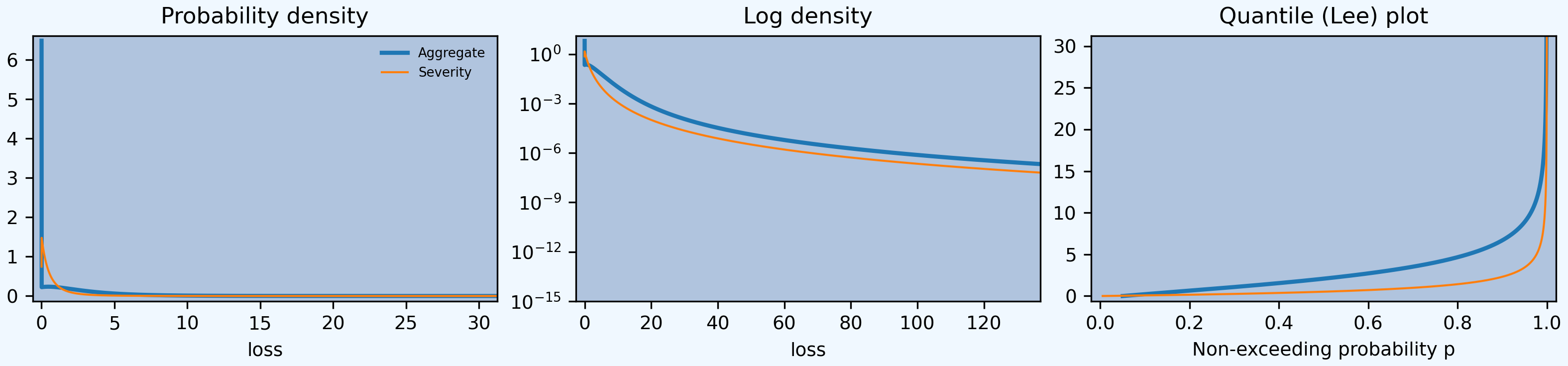
In [91]: kpw_9_14.plot()
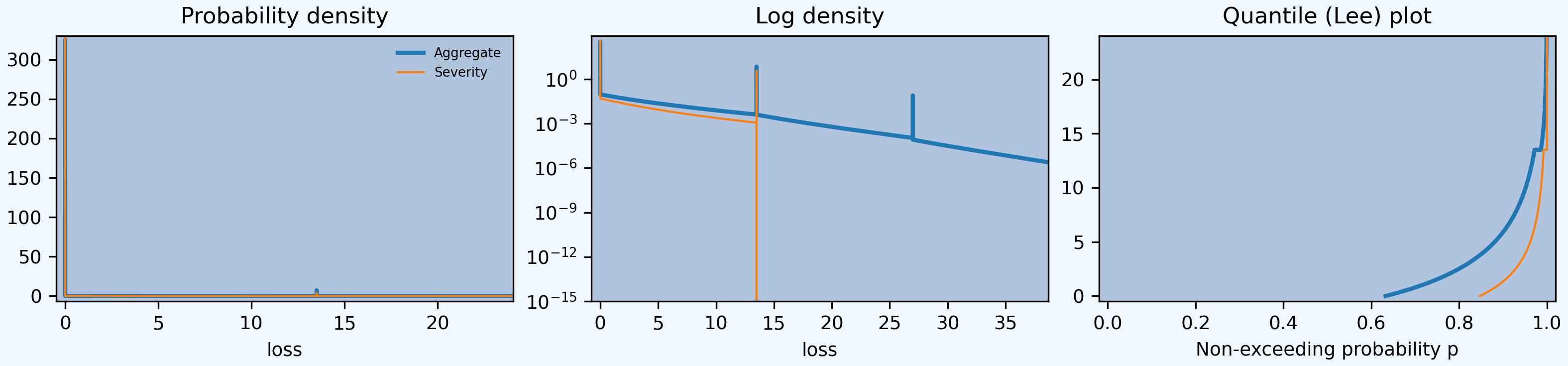
describe returns gross under E[X] and the requested net or ceded under Est E[X]. The print statement computes net variance from the product of estimated mean and cv. The spikes on the density corresponds to the possibility of only limit claims.
Exercise 9.63. A ground-up model of individual losses has a gamma distribution with shape parameter 2 and scale 100. The number of losses has a negative binomial distribution with \(r = 2\) and \(\beta = 1.5\). An ordinary deductible of 50 and a loss limit of 175 (before imposition of the deductible) are applied to each individual loss.
Determine the mean and variance of the aggregate payments on a per-loss basis.
Determine the distribution of the number of payments.
Determine the cumulative distribution function of the amount of a payment, given that a payment is made.
Discretize the severity distribution using the method of rounding and a span of 40.
Calculate the discretized distribution of aggregate payments up to a discretized amount paid of 120.
Negative binomial \(c=1/2\) and hence mixing cv \(\sqrt{c}\), and the mean equals \(r\beta/(1+\beta)=1.4\). The cover is 125 xs 50. The severity is unconditional. First, the default calculation using bs=1/64.
In [92]: kpw_9_63 = build('agg KPW.9.63 1.4 claims '
   ....:                  '125 xs 50 '
   ....:                  'sev 100 * gamma 2 ! '
   ....:                  'mixed gamma 2**-0.5')
   ....:

In [93]: qd(kpw_9_63)

       E[X] Est E[X]    Err E[X]   CV(X) Est CV(X)  Skew(X) Est Skew(X)
X
Freq    1.4                       1.1019             1.5557
Sev  86.467   86.467  3.9488e-12 0.54006   0.54006 -0.74977    -0.74977
Agg  121.05   121.05 -3.9543e-08  1.1927    1.1927   1.6385      1.6385
log2 = 16, bandwidth = 1/32, validation: fails agg mean error >> sev, possible aliasing; try larger bs.

In [94]: mv(kpw_9_63)
mean     = 121.054
variance = 20847.33
std dev  = 144.386

In [95]: qd(kpw_9_63.density_df.loc[:400:40*64,
   ....:     ['p', 'F', 'S', 'p_sev', 'F_sev', 'S_sev']],
   ....:     accuracy=5)
   ....:

               p       F        S      p_sev    F_sev   S_sev
loss
0.0      0.37325 0.37325  0.62675   0.090251 0.090251 0.90975
80.0  4.2253e-05 0.47185  0.52815 0.00011072  0.37323 0.62677
160.0  3.327e-05 0.72045  0.27955          0        1       0
240.0 3.0211e-05 0.80373  0.19627          0        1       0
320.0 1.7591e-05  0.9016 0.098397          0        1       0
400.0 9.0878e-06 0.94991 0.050095          0        1       0
Next, calculations performed with the requested broader bs=40.
In [96]: kpw_9_63.update(log2=8, bs=40)

In [97]: qd(kpw_9_63)

       E[X] Est E[X] Err E[X]   CV(X) Est CV(X)  Skew(X) Est Skew(X)
X
Freq    1.4                    1.1019             1.5557
Sev  86.467   84.042 -0.02805 0.54006     0.546 -0.74977    -0.81723
Agg  121.05   117.66 -0.02805  1.1927    1.1947   1.6385       1.636
log2 = 8, bandwidth = 40, validation: fails sev mean, agg mean.

In [98]: qd(kpw_9_63.density_df.loc[:400,
   ....:     ['p', 'F', 'S', 'p_sev', 'F_sev', 'S_sev']],
   ....:     accuracy=5)
   ....:

             p       F        S   p_sev   F_sev   S_sev
loss
0.0    0.39509 0.39509  0.60491  0.1558  0.1558  0.8442
40.0   0.05047 0.44556  0.55444 0.14517 0.30097 0.69903
80.0  0.053928 0.49949  0.50051  0.1412 0.44217 0.55783
120.0  0.20376 0.70325  0.29675 0.55783       1       0
160.0 0.042972 0.74622  0.25378       0       1       0
200.0 0.042194 0.78841  0.21159       0       1       0
240.0 0.081719 0.87013  0.12987       0       1       0
280.0 0.024403 0.89453  0.10547       0       1       0
320.0  0.02234 0.91687 0.083127       0       1       0
360.0 0.030181 0.94705 0.052946       0       1       0
400.0 0.011572 0.95863 0.041374       0       1       0
The apparent difference in the severity distribution is caused by the rounding method. In the first case F(40) is almost exact whereas in the second it is actually F(60).
2.13.5.8. Group Life Individual Risk Model, Example 9.15, 9.18
Consider a group life insurance contract with an accidental death benefit. Assume that for all members the probability of death in the next year is 0.01 and that 30% of deaths are accidental. For 50 employees, the benefit for an ordinary death is 50,000 and for an accidental death it is 100,000. For the remaining 25 employees, the benefits are 75,000 and 150,000, respectively. Develop an individual risk model and determine its mean and variance.
The Portfolio solution, working in thousands.
In [99]: kpw_9_15p = build('port KPW.9.15.p '
   ....:                   'agg A 0.5 claims '
   ....:                       'dsev [50 100] [0.7 0.3] '
   ....:                       'binomial 0.01 '
   ....:                   'agg B 0.25 claims '
   ....:                       'dsev [75 150] [0.7 0.3] '
   ....:                       'binomial 0.01 ')
   ....:

In [100]: qd(kpw_9_15p)

             E[X] Est E[X]    Err E[X]   CV(X) Est CV(X)  Skew(X) Est Skew(X)
unit  X
A     Freq    0.5                       1.4071             1.3929
      Sev      65       65           0 0.35251   0.35251  0.87287     0.87287
      Agg    32.5     32.5    2.82e-14  1.4928    1.4928   1.6562      1.6562
B     Freq   0.25                         1.99             1.9699
      Sev    97.5     97.5           0 0.35251   0.35251  0.87287     0.87287
      Agg  24.375   24.375  1.1613e-13  2.1112    2.1112   2.3423      2.3423
total Freq   0.75                       1.1489             1.1373
      Sev  75.833   75.833           0 0.41249             1.1623
      Agg  56.875   56.875 -8.6597e-15  1.2435    1.2435   1.4369      1.4369
log2 = 16, bandwidth = 1/16, validation: not unreasonable.

In [101]: mv(kpw_9_15p)
mean     = 56.875
variance = 5001.984
std dev  = 70.7247
The density_df dataframe contains the exact aggregate distribution, which is not easy to compute by other means. KPW says (emphasis added)
With regard to calculating the probabilities, there are at least three options. One is to do an exact calculation, which involves numerous convolutions and almost always requires more excessive computing time. Recursive formulas have been developed, but they are cumbersome and are not presented here. For one such method, see De Pril [27]. One alternative is a parametric approximation as discussed for the collective risk model. Another alternative is to replace the individual risk model with a similar collective risk model and then do the calculations with that model. These two approaches are presented here.
The following solution attempts to commute convolution through the mixture. This works for a compound Poisson. However, the sum of binomials is not binomial, and so the frequencies can’t be independent binomial. They can be independent Poisson because it is additive.
In [102]: kpw_9_15w = build('agg KPW.9.15.w '
   .....:                  '0.75 claims '
   .....:                  'dsev [50 75 100 150] '
   .....:                  '[0.35/0.75, 0.175/0.75, 0.15/0.75, 0.075/0.75] '
   .....:                  'binomial 0.01 ')
   .....:

In [103]: qd(kpw_9_15w)

       E[X] Est E[X]    Err E[X]   CV(X) Est CV(X)  Skew(X) Est Skew(X)
X
Freq   0.75                       1.1489             1.1373
Sev  75.833   75.833  2.2204e-16 0.41249   0.41249   1.1623      1.1623
Agg  56.875   56.875 -6.9356e-11  1.2437    1.2437   1.4389      1.4389
log2 = 10, bandwidth = 1, validation: fails agg mean error >> sev, possible aliasing; try larger bs.

In [104]: mv(kpw_9_15w)
mean     = 56.875
variance = 5003.745
std dev  = 70.7372
The compound Poisson approximation matches the mean but its variance is slightly off.
In [105]: kpw_9_15cp = build('agg KPW.9.15.cp '
   .....:                  '0.75 claims '
   .....:                  'dsev [50 75 100 150] '
   .....:                  '[0.35/0.75, 0.175/0.75, 0.15/0.75, 0.075/0.75] '
   .....:                  'poisson ')
   .....:

In [106]: qd(kpw_9_15cp)

       E[X] Est E[X]    Err E[X]   CV(X) Est CV(X)  Skew(X) Est Skew(X)
X
Freq   0.75                       1.1547             1.1547
Sev  75.833   75.833  2.2204e-16 0.41249   0.41249   1.1623      1.1623
Agg  56.875   56.875 -1.1396e-10  1.2491    1.2491   1.4523      1.4523
log2 = 10, bandwidth = 1, validation: fails agg mean error >> sev, possible aliasing; try larger bs.

In [107]: mv(kpw_9_15cp)
mean     = 56.875
variance = 5046.875
std dev  = 71.0414
Comparing probabilities shows that all three distributions are very close.
In [108]: bit = pd.concat((kpw_9_15p.density_df.loc[:400:128, ['p_total']].query('p_total > 1e-10'),
   .....:                  kpw_9_15cp.density_df.loc[:400, ['p_total']].query('p_total > 0'),
   .....:                  kpw_9_15w.density_df.loc[:400, ['p_total']].query('p_total > 0'),
   .....:                 ),
   .....:                 keys=('exact', 'compound Po', 'wrong'), axis=1).rename(columns={'p_total': 'p'})
   .....:

In [109]: bit = bit.droplevel(1, axis=1)

In [110]: bit.index.name = 'loss'

In [111]: qd(bit, accuracy=5)

           exact  compound Po      wrong
loss
0.0      0.47059      0.47237    0.47059
200.0   0.024856     0.024881   0.024823
400.0 0.00061615   0.00064447 0.00061581
50.0         NaN      0.16533    0.16637
75.0         NaN     0.082664   0.083185
100.0        NaN     0.099787    0.10032
125.0        NaN     0.028932   0.029017
150.0        NaN     0.070835   0.071104
175.0        NaN     0.017463   0.017428
225.0        NaN     0.011552   0.011478
250.0        NaN     0.011399     0.0113
275.0        NaN    0.0040587  0.0039712
300.0        NaN    0.0050707   0.004986
325.0        NaN    0.0018166  0.0017595
350.0        NaN     0.001694  0.0016392
375.0        NaN   0.00077117 0.00073805
2.13.5.9. Group Life Individual Risk Model, Example 9.16, 9.17
A small manufacturing business has a group life insurance contract on its 14 permanent employees. The actuary for the insurer has selected a mortality table to represent the mortality of the group. Each employee is insured for the amount of his or her salary rounded up to the next 1,000. The group’s data are shown in the next table.
If the insurer adds a 45% relative loading to the net (pure) premium, what are the chances that it will lose money in a given year? Use the normal and lognormal approximations.
In order to make the answer self-contained, the code below includes the data munging to re-create the table, pasted from a pdf.
In [112]: data = '''1
   .....: 20
   .....: M
   .....: 15,000
   .....: 0.00149
   .....: 2
   .....: 23
   .....: M
   .....: 16,000
   .....: 0.00142
   .....: 3
   .....: 27
   .....: M
   .....: 20,000
   .....: 0.00128
   .....: 4
   .....: 30
   .....: M
   .....: 28,000
   .....: 0.00122
   .....: 5
   .....: 31
   .....: M
   .....: 31,000
   .....: 0.00123
   .....: 6
   .....: 46
   .....: M
   .....: 18,000
   .....: 0.00353
   .....: 7
   .....: 47
   .....: M
   .....: 26,000
   .....: 0.00394
   .....: 8
   .....: 49
   .....: M
   .....: 24,000
   .....: 0.00484
   .....: 9
   .....: 64
   .....: M
   .....: 60,000
   .....: 0.02182
   .....: 10
   .....: 17
   .....: F
   .....: 14,000
   .....: 0.00050
   .....: 11
   .....: 22
   .....: F
   .....: 17,000
   .....: 0.00050
   .....: 12
   .....: 26
   .....: F
   .....: 19,000
   .....: 0.00054
   .....: 13
   .....: 37
   .....: F
   .....: 30,000
   .....: 0.00103
   .....: 14
   .....: 55
   .....: F
   .....: 55,000
   .....: 0.00479'''
   .....:

In [113]: sdata = data.split('\n')

In [114]: df = pd.DataFrame(zip(*[iter(sdata)]*5),
   .....:                   columns=['Employee', 'Age', 'Sex', 'Benefit', 'q'])
   .....:

In [115]: df.Benefit = df.Benefit.str.replace(',','').astype(float)

In [116]: df.q = df.q.astype(float)

In [117]: df = df.set_index('Employee')

In [118]: qd(df)

         Age Sex  Benefit       q
Employee
1         20   M    15000 0.00149
2         23   M    16000 0.00142
3         27   M    20000 0.00128
4         30   M    28000 0.00122
5         31   M    31000 0.00123
6         46   M    18000 0.00353
7         47   M    26000 0.00394
8         49   M    24000 0.00484
9         64   M    60000 0.02182
10        17   F    14000  0.0005
11        22   F    17000  0.0005
12        26   F    19000 0.00054
13        37   F    30000 0.00103
14        55   F    55000 0.00479

In [119]: print(f'expected claim count = {df.q.sum():.6g}')
expected claim count = 0.04813
Here are the FFT-exact, and various approximations to the required probability. Working in thousands. The dsev clauses enter the fixed benefit amount for each employee. Note the outsize impact of employee 9.
In [120]: from aggregate import Portfolio

In [121]: a = [build(f'agg ee.{i} {r.q} claims '
   .....:            f'dsev [{r.Benefit / 1000}] '
   .....:            f'bernoulli')
   .....:          for i, r in df.iterrows()]
   .....:

In [122]: kpw_9_16p = Portfolio('KPW.9.16p', a)

In [123]: kpw_9_16p.update(log2=8, bs=1, remove_fuzz=True)

In [124]: qd(kpw_9_16p)

              E[X] Est E[X]    Err E[X]   CV(X) Est CV(X)  Skew(X) Est Skew(X)
unit  X
ee.1  Freq 0.00149                       25.887             25.848
      Sev       15       15 -1.1102e-16       0         0
      Agg  0.02235  0.02235  8.8818e-16  25.887    25.887   25.848      25.848
ee.2  Freq 0.00142                       26.518             26.481
      Sev       16       16           0       0         0
      Agg  0.02272  0.02272  -1.481e-13  26.518    26.518   26.481      26.481
ee.3  Freq 0.00128                       27.933             27.897
      Sev       20       20           0       0         0
      Agg   0.0256   0.0256 -8.7597e-14  27.933    27.933   27.897      27.897
ee.4  Freq 0.00122                       28.612             28.577
      Sev       28       28  2.2204e-16       0         0
      Agg  0.03416  0.03416   3.908e-14  28.612    28.612   28.577      28.577
...            ...      ...         ...     ...       ...      ...         ...
ee.12 Freq 0.00054                       43.022             42.998
      Sev       19       19           0       0         0
      Agg  0.01026  0.01026    1.35e-13  43.022    43.022   42.998      42.998
ee.13 Freq 0.00103                       31.143             31.111
      Sev       30       30           0       0         0
      Agg   0.0309   0.0309 -4.2188e-15  31.143    31.143   31.111      31.111
ee.14 Freq 0.00479                       14.414             14.345
      Sev       55       55 -1.1102e-16       0         0
      Agg  0.26345  0.26345 -2.1538e-14  14.414    14.414   14.345      14.345
total Freq 0.04813                       4.5315             4.4789
      Sev   42.685   42.685           0 0.43586           -0.28928
      Agg   2.0544   2.0544 -5.9397e-14  4.9289    4.9289   5.2673      5.2673
log2 = 8, bandwidth = 1, validation: not unreasonable.

In [125]: mv(kpw_9_16p)
mean     = 2.05441
variance = 102.5336
std dev  = 10.1259

In [126]: appx = kpw_9_16p.approximate('all')

In [127]: premium = 1.45 * kpw_9_16p.agg_m

In [128]: ans = {k: v.sf(premium) for k, v in appx.items()}

In [129]: ans['FFT'] = kpw_9_16p.sf(premium)

In [130]: qd(pd.DataFrame(ans.values(),
   .....:                 index=pd.Index(ans.keys(), name='method'),
   .....:                 columns=['premium']).sort_values('premium'),
   .....:   accuracy=5)
   .....:

          premium
method
FFT      0.047261
gamma    0.091498
lognorm   0.13449
sgamma    0.18346
slognorm  0.28099
norm      0.46363
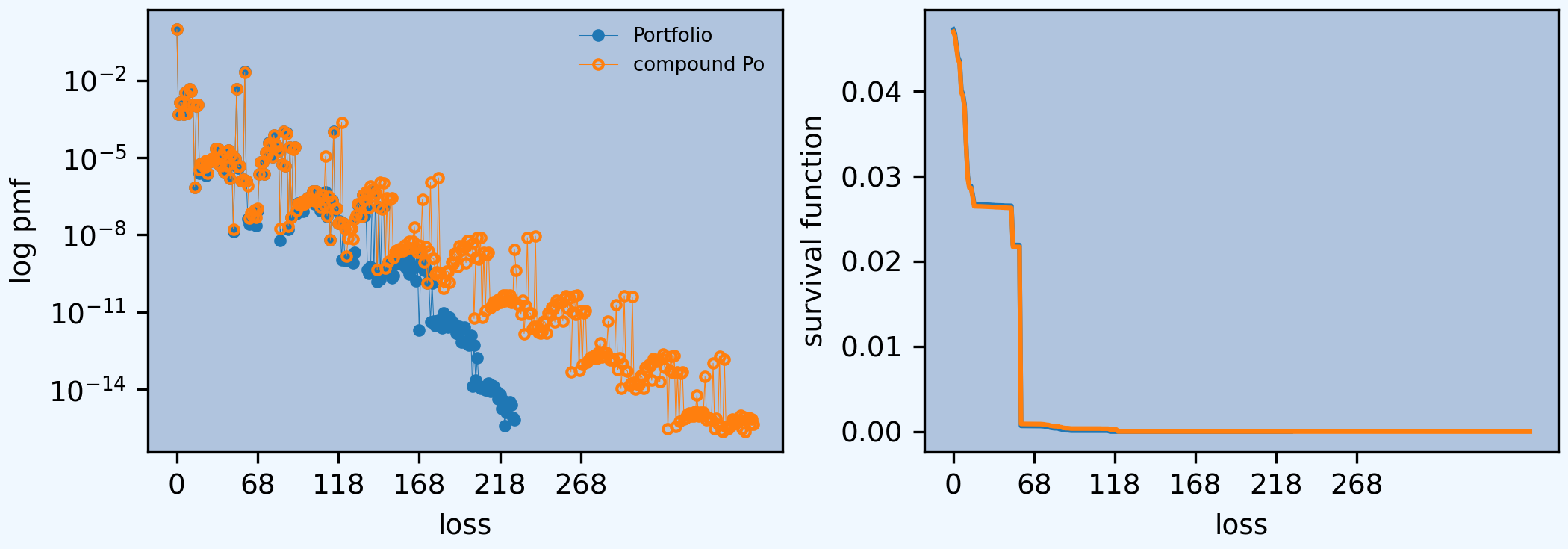
Here is a sample from the distribution and the mean-matched compound Poisson (for Exercise 9.18). The latter dsev clause works because all the benefit amounts are different. The temporary variable sev creates the severity curve. The log pmf graph reflects the irregular benefit amounts. Compare the cdf under comp Po with Table 9.17.
In [131]: sev = df[['Benefit', 'q']]
In [132]: sev.q = sev.q / sev.q.sum()
In [133]: sev = sev.sort_values('Benefit')
In [134]: kpw_9_16cp = build('agg kpw_9_16.po '
.....: f'{df.q.sum()} claims '
.....: f'dsev {sev.Benefit.values / 1000} {sev.q.values} '
.....: 'poisson', bs=1, log2=10)
.....:
In [135]: qd(kpw_9_16cp)
E[X] Est E[X] Err E[X] CV(X) Est CV(X) Skew(X) Est Skew(X)
X
Freq 0.04813 4.5582 4.5582
Sev 42.685 42.685 0 0.43586 0.43586 -0.28928 -0.28928
Agg 2.0544 2.0544 3.4417e-14 4.9723 4.9723 5.4286 5.4286
log2 = 10, bandwidth = 1, validation: not unreasonable.
In [136]: bit = pd.concat((kpw_9_16p.density_df.query('p_total > 0')[['p_total', 'F', 'S']],
.....: kpw_9_16cp.density_df.query('p_total > 0')[['p_total', 'F', 'S']]),
.....: keys=['exact', 'comp Po'], axis=1)
.....:
In [137]: bit.index = [f'{i:.0f}' for i in bit.index]
In [138]: bit.index.name = 'loss'
In [139]: with pd.option_context('display.max_rows', 360, 'display.max_columns', 10,
.....: 'display.width', 150, 'display.float_format', lambda x: f'{x:.7g}'):
.....: print(bit)
.....:
exact comp Po
p_total F S p_total F S
loss
0 0.952739 0.952739 0.04726095 0.9530099 0.9530099 0.04699011
14 0.0004766078 0.9532157 0.04678434 0.0004765049 0.9534864 0.04651361
15 0.0014217 0.9546374 0.04536264 0.001419985 0.9549064 0.04509362
16 0.001354813 0.9559922 0.04400783 0.001353274 0.9562597 0.04374035
17 0.0004766078 0.9564688 0.04353122 0.0004765049 0.9567362 0.04326384
18 0.003375083 0.9598439 0.04015614 0.003364125 0.9601003 0.03989972
19 0.0005147571 0.9603586 0.03964138 0.0005146252 0.9606149 0.03938509
20 0.001221069 0.9615797 0.03842031 0.001219853 0.9618348 0.03816524
24 0.004633684 0.9662134 0.03378663 0.004612568 0.9664473 0.03355267
26 0.00376864 0.969982 0.03001799 0.003754859 0.9702022 0.02979781
28 0.001163761 0.9711458 0.02885423 0.001162791 0.971365 0.02863502
29 7.112054e-07 0.9711465 0.02885352 7.099922e-07 0.9713657 0.02863431
30 0.0009830108 0.9721295 0.02787051 0.0009833345 0.972349 0.02765098
31 0.001175572 0.9733051 0.02669493 0.001174457 0.9735235 0.02647652
32 2.399591e-06 0.9733075 0.02669253 3.352879e-06 0.9735268 0.02647317
33 5.971631e-06 0.9733134 0.02668656 5.946495e-06 0.9735328 0.02646722
34 6.178405e-06 0.9733196 0.02668038 6.272902e-06 0.9735391 0.02646095
35 4.242488e-06 0.9733239 0.02667614 4.23041e-06 0.9735433 0.02645672
36 1.993891e-06 0.9733259 0.02667415 7.927184e-06 0.9735512 0.02644879
37 2.434369e-06 0.9733283 0.02667171 2.426553e-06 0.9735536 0.02644637
38 6.643644e-06 0.9733349 0.02666507 6.751312e-06 0.9735604 0.02643961
39 7.574225e-06 0.9733425 0.02665749 7.531446e-06 0.9735679 0.02643208
40 8.474451e-06 0.973351 0.02664902 9.207982e-06 0.9735771 0.02642287
41 7.941654e-06 0.9733589 0.02664108 7.901023e-06 0.973585 0.02641497
42 2.23561e-05 0.9733813 0.02661872 2.219562e-05 0.9736072 0.02639278
43 6.125396e-06 0.9733874 0.0266126 6.100774e-06 0.9736133 0.02638668
44 2.143545e-05 0.9734088 0.02659116 2.130123e-05 0.9736346 0.02636538
45 4.672158e-06 0.9734135 0.02658649 4.659237e-06 0.9736393 0.02636072
46 1.210077e-05 0.9734256 0.02657439 1.205366e-05 0.9736513 0.02634866
47 2.791514e-06 0.9734284 0.0265716 2.78804e-06 0.9736541 0.02634587
48 5.56219e-06 0.973434 0.02656603 1.670997e-05 0.9736708 0.02632916
49 4.696495e-06 0.9734387 0.02656134 4.6784e-06 0.9736755 0.02632449
50 2.022647e-05 0.9734589 0.02654111 2.007543e-05 0.9736956 0.02630441
51 1.510358e-06 0.9734604 0.0265396 1.516371e-06 0.9736971 0.02630289
52 5.666162e-06 0.9734661 0.02653394 1.304127e-05 0.9737101 0.02628985
53 1.370555e-08 0.9734661 0.02653392 1.686769e-08 0.9737102 0.02628984
54 9.392317e-06 0.9734755 0.02652453 9.356468e-06 0.9737195 0.02628048
55 0.004591308 0.9780668 0.02193322 0.004570612 0.9782901 0.02170987
56 3.900383e-06 0.9780707 0.02192932 4.60947e-06 0.9782947 0.02170526
57 4.682325e-06 0.9780754 0.02192464 4.659748e-06 0.9782994 0.0217006
58 1.240279e-06 0.9780766 0.0219234 1.246296e-06 0.9783006 0.02169935
59 1.480938e-06 0.9780781 0.02192192 1.478042e-06 0.9783021 0.02169787
60 0.02125253 0.9993306 0.000669383 0.02079525 0.9990974 0.0009026226
61 1.248838e-06 0.9993319 0.0006681341 1.247493e-06 0.9990986 0.0009013751
62 4.172979e-08 0.9993319 0.0006680924 7.93117e-07 0.9990994 0.000900582
63 2.713599e-08 0.9993319 0.0006680653 4.479884e-08 0.9990995 0.0009005372
64 4.244129e-08 0.999332 0.0006680228 6.96877e-08 0.9990995 0.0009004675
65 4.491981e-08 0.999332 0.0006679779 5.030504e-08 0.9990996 0.0009004172
66 4.146533e-08 0.9993321 0.0006679364 9.361181e-08 0.9990997 0.0009003236
67 2.339189e-08 0.9993321 0.000667913 4.760197e-08 0.9990997 0.000900276
68 8.513895e-08 0.9993322 0.0006678279 1.101497e-07 0.9990998 0.0009001659
69 2.329551e-06 0.9993345 0.0006654983 2.321713e-06 0.9991022 0.0008978441
70 6.910878e-06 0.9993414 0.0006585875 6.89662e-06 0.9991091 0.0008909475
71 6.544798e-06 0.999348 0.0006520427 6.512085e-06 0.9991156 0.0008844354
72 2.350356e-06 0.9993503 0.0006496923 2.366974e-06 0.9991179 0.0008820685
73 1.628085e-05 0.9993666 0.0006334115 1.615066e-05 0.9991341 0.0008659178
74 1.314419e-05 0.9993797 0.0006202673 1.294404e-05 0.999147 0.0008529738
75 3.761971e-05 0.9994174 0.0005826475 3.685732e-05 0.9991839 0.0008161165
76 3.023577e-05 0.9994476 0.0005524118 2.959418e-05 0.9992135 0.0007865223
77 1.064505e-05 0.9994582 0.0005417667 1.041214e-05 0.9992239 0.0007761101
78 7.531246e-05 0.9995335 0.0004664543 7.34545e-05 0.9992973 0.0007026556
79 3.379094e-05 0.9995673 0.0004326633 3.334395e-05 0.9993307 0.0006693117
80 2.725768e-05 0.9995946 0.0004054057 2.665243e-05 0.9993573 0.0006426592
81 1.816289e-05 0.9996128 0.0003872428 1.801028e-05 0.9993754 0.000624649
82 5.911614e-09 0.9996128 0.0003872369 1.74019e-08 0.9993754 0.0006246316
83 5.608384e-06 0.9996184 0.0003816285 5.586048e-06 0.999381 0.0006190455
84 0.0001033707 0.9997217 0.0002782578 0.0001006574 0.9994816 0.0005183881
85 4.743e-06 0.9997265 0.0002735148 4.72191e-06 0.9994863 0.0005136662
86 8.972427e-05 0.9998162 0.0001837905 8.756326e-05 0.9995739 0.0004261029
87 1.649612e-08 0.9998162 0.000183774 2.194197e-08 0.9995739 0.000426081
88 2.598867e-05 0.9998422 0.0001577853 2.540443e-05 0.9995993 0.0004006766
89 4.722525e-08 0.9998423 0.0001577381 4.726622e-08 0.9995994 0.0004006293
90 2.194831e-05 0.9998642 0.0001357898 2.147808e-05 0.9996208 0.0003791512
91 2.623287e-05 0.9998904 0.0001095569 2.56655e-05 0.9996465 0.0003534857
92 6.536066e-08 0.9998905 0.0001094916 8.594597e-08 0.9996466 0.0003533998
93 1.65287e-07 0.9998907 0.0001093263 1.62614e-07 0.9996468 0.0003532372
94 1.743665e-07 0.9998908 0.0001091519 1.733535e-07 0.9996469 0.0003530638
95 1.355125e-07 0.999891 0.0001090164 1.365987e-07 0.9996471 0.0003529272
96 8.286137e-08 0.9998911 0.0001089335 2.111788e-07 0.9996473 0.000352716
97 1.619798e-07 0.9998912 0.0001087716 1.594421e-07 0.9996474 0.0003525566
98 1.778121e-07 0.9998914 0.0001085938 1.768561e-07 0.9996476 0.0003523797
99 2.722478e-07 0.9998917 0.0001083215 2.665397e-07 0.9996479 0.0003521132
100 2.116102e-07 0.9998919 0.0001081099 2.234979e-07 0.9996481 0.0003518897
101 2.354722e-07 0.9998921 0.0001078744 2.302657e-07 0.9996483 0.0003516594
102 5.121685e-07 0.9998926 0.0001073623 4.978643e-07 0.9996488 0.0003511616
103 1.63469e-07 0.9998928 0.0001071988 2.132647e-07 0.9996491 0.0003509483
104 5.007765e-07 0.9998933 0.000106698 4.873585e-07 0.9996495 0.0003504609
105 2.016058e-07 0.9998935 0.0001064964 1.979245e-07 0.9996497 0.000350263
106 2.772016e-07 0.9998938 0.0001062192 2.703786e-07 0.99965 0.0003499926
107 8.955276e-08 0.9998939 0.0001061296 1.233815e-07 0.9996501 0.0003498692
108 1.241644e-07 0.999894 0.0001060055 3.6475e-07 0.9996505 0.0003495045
109 1.499989e-07 0.9998941 0.0001058555 1.469601e-07 0.9996506 0.0003493575
110 4.787335e-07 0.9998946 0.0001053768 1.139834e-05 0.999662 0.0003379592
111 5.24875e-08 0.9998947 0.0001053243 5.520826e-08 0.9996621 0.000337904
112 1.489302e-07 0.9998948 0.0001051753 3.069069e-07 0.9996624 0.0003375971
113 6.282775e-09 0.9998948 0.0001051691 6.359186e-09 0.9996624 0.0003375907
114 2.166401e-07 0.999895 0.0001049524 2.112529e-07 0.9996626 0.0003373795
115 0.0001024173 0.9999975 2.53513e-06 9.973353e-05 0.9997624 0.0002376459
116 9.301591e-08 0.9999976 2.442114e-06 1.065637e-07 0.9997625 0.0002375394
117 1.046485e-07 0.9999977 2.337466e-06 1.054805e-07 0.9997626 0.0002374339
118 2.779748e-08 0.9999977 2.309668e-06 2.74138e-08 0.9997626 0.0002374065
119 3.323942e-08 0.9999977 2.276429e-06 3.258744e-08 0.9997626 0.0002373739
120 1.07834e-09 0.9999977 2.27535e-06 0.0002268827 0.9999895 1.049118e-05
121 2.805718e-08 0.9999978 2.247293e-06 2.767002e-08 0.9999895 1.046351e-05
122 1.04354e-09 0.9999978 2.24625e-06 1.753529e-08 0.9999896 1.044597e-05
123 1.015218e-09 0.9999978 2.245234e-06 1.506102e-09 0.9999896 1.044447e-05
124 1.11823e-09 0.9999978 2.244116e-06 7.176094e-09 0.9999896 1.043729e-05
125 1.330164e-09 0.9999978 2.242786e-06 1.78429e-08 0.9999896 1.041945e-05
126 1.040647e-09 0.9999978 2.241745e-06 1.771138e-08 0.9999896 1.040174e-05
127 7.934845e-10 0.9999978 2.240952e-06 6.910456e-09 0.9999896 1.039483e-05
128 2.074415e-09 0.9999978 2.238878e-06 4.117227e-08 0.9999896 1.035365e-05
129 5.213364e-08 0.9999978 2.186744e-06 5.695507e-08 0.9999897 1.02967e-05
130 1.542995e-07 0.999998 2.032444e-06 1.646233e-07 0.9999899 1.013208e-05
131 1.46062e-07 0.9999981 1.886382e-06 1.424089e-07 0.99999 9.989666e-06
132 5.249366e-08 0.9999982 1.833889e-06 5.171857e-08 0.9999901 9.937948e-06
133 3.632949e-07 0.9999985 1.470594e-06 3.526438e-07 0.9999904 9.585304e-06
134 5.60785e-08 0.9999986 1.414515e-06 2.220186e-07 0.9999906 9.363285e-06
135 1.318434e-07 0.9999987 1.282672e-06 4.663595e-07 0.9999911 8.896926e-06
136 4.358886e-10 0.9999987 1.282236e-06 3.667832e-07 0.9999915 8.530142e-06
137 3.292504e-10 0.9999987 1.281907e-06 1.138415e-07 0.9999916 8.416301e-06
138 6.005527e-10 0.9999987 1.281306e-06 8.153441e-07 0.9999924 7.600957e-06
139 4.976509e-07 0.9999992 7.836552e-07 6.051008e-07 0.999993 6.995856e-06
140 4.940901e-10 0.9999992 7.831612e-07 3.024997e-07 0.9999933 6.693356e-06
141 4.051553e-07 0.9999996 3.780058e-07 4.064893e-07 0.9999937 6.286867e-06
142 1.556782e-10 0.9999996 3.778501e-07 4.463796e-10 0.9999937 6.286421e-06
143 1.251058e-07 0.9999997 2.527444e-07 1.219742e-07 0.9999938 6.164447e-06
144 1.937367e-10 0.9999997 2.525506e-07 1.098375e-06 0.9999949 5.066072e-06
145 1.058015e-07 0.9999999 1.467492e-07 1.030876e-07 0.999995 4.962984e-06
146 1.262168e-07 1 2.053237e-08 1.016858e-06 0.9999961 3.946126e-06
147 3.685373e-10 1 2.016383e-08 5.121882e-10 0.9999961 3.945614e-06
148 6.46479e-10 1 1.951735e-08 2.77595e-07 0.9999963 3.668019e-06
149 6.999917e-10 1 1.881736e-08 9.506666e-10 0.9999963 3.667068e-06
150 4.588675e-10 1 1.835849e-08 2.346692e-07 0.9999966 3.432399e-06
151 2.170583e-10 1 1.814144e-08 2.805268e-07 0.9999968 3.151872e-06
152 2.643346e-10 1 1.78771e-08 1.33265e-09 0.9999968 3.15054e-06
153 7.16224e-10 1 1.716088e-08 2.204159e-09 0.9999969 3.148335e-06
154 8.158174e-10 1 1.634506e-08 2.534458e-09 0.9999969 3.145801e-06
155 9.122321e-10 1 1.543283e-08 2.028215e-09 0.9999969 3.143773e-06
156 8.566022e-10 1 1.457623e-08 2.859701e-09 0.9999969 3.140913e-06
157 2.40212e-09 1 1.217411e-08 2.93432e-09 0.9999969 3.137979e-06
158 6.608837e-10 1 1.151322e-08 2.44401e-09 0.9999969 3.135535e-06
159 2.304181e-09 1 9.209041e-09 4.077408e-09 0.9999969 3.131457e-06
160 5.036921e-10 1 8.705349e-09 2.915487e-09 0.9999969 3.128542e-06
161 1.300943e-09 1 7.404406e-09 3.161405e-09 0.9999969 3.12538e-06
162 3.006818e-10 1 7.103724e-09 5.729582e-09 0.9999969 3.119651e-06
163 5.986384e-10 1 6.505086e-09 3.201579e-09 0.9999969 3.116449e-06
164 5.047601e-10 1 6.000326e-09 5.670897e-09 0.9999969 3.110778e-06
165 2.172347e-09 1 3.827979e-09 2.073139e-08 0.9999969 3.090047e-06
166 1.623502e-10 1 3.665628e-09 3.083291e-09 0.9999969 3.086964e-06
167 6.086006e-10 1 3.057028e-09 2.082057e-09 0.9999969 3.084882e-06
168 2.04573e-12 1 3.054982e-09 3.995334e-09 0.9999969 3.080886e-06
169 1.009057e-09 1 2.045925e-09 2.109975e-09 0.9999969 3.078776e-06
170 6.145147e-10 1 1.431411e-09 2.439393e-07 0.9999972 2.834837e-06
171 4.192868e-10 1 1.012124e-09 8.580199e-10 0.9999972 2.833979e-06
172 5.027193e-10 1 5.094045e-10 3.601279e-09 0.9999972 2.830378e-06
173 1.333299e-10 1 3.760746e-10 1.352801e-10 0.9999972 2.830242e-06
174 1.590085e-10 1 2.170661e-10 2.382985e-09 0.9999972 2.827859e-06
175 4.288268e-12 1 2.127779e-10 1.088124e-06 0.9999983 1.739736e-06
176 1.340885e-10 1 7.868939e-11 1.228987e-09 0.9999983 1.738507e-06
177 4.486189e-12 1 7.42032e-11 1.192855e-09 0.9999983 1.737314e-06
178 2.920835e-12 1 7.128231e-11 3.02749e-10 0.9999983 1.737011e-06
179 4.562823e-12 1 6.671952e-11 3.683841e-10 0.9999983 1.736643e-06
180 4.82662e-12 1 6.189294e-11 1.65027e-06 0.9999999 8.637285e-08
181 4.454919e-12 1 5.743805e-11 3.319206e-10 0.9999999 8.604093e-08
182 2.514367e-12 1 5.492373e-11 2.035136e-10 0.9999999 8.583741e-08
183 9.143925e-12 1 4.577982e-11 8.424069e-11 0.9999999 8.575317e-08
184 3.826298e-12 1 4.195355e-11 1.503577e-10 0.9999999 8.560282e-08
185 7.320083e-12 1 3.463352e-11 4.000487e-10 0.9999999 8.520277e-08
186 2.580997e-12 1 3.205247e-11 3.64933e-10 0.9999999 8.483783e-08
187 6.060502e-12 1 2.599199e-11 1.396254e-10 0.9999999 8.469821e-08
188 3.909234e-12 1 2.208278e-11 8.727237e-10 0.9999999 8.382548e-08
189 3.768936e-12 1 1.831379e-11 7.747876e-10 0.9999999 8.30507e-08
190 3.132506e-12 1 1.51813e-11 1.950703e-09 0.9999999 8.109999e-08
191 1.538332e-12 1 1.364298e-11 1.62618e-09 0.9999999 7.947381e-08
192 1.447886e-12 1 1.219513e-11 5.652266e-10 0.9999999 7.890859e-08
193 2.725839e-12 1 9.469314e-12 3.871408e-09 0.9999999 7.503718e-08
194 6.673824e-13 1 8.801959e-12 2.58819e-09 0.9999999 7.244899e-08
195 2.106876e-12 1 6.695089e-12 3.878648e-09 0.9999999 6.857034e-08
196 2.600251e-12 1 4.094836e-12 3.322862e-09 0.9999999 6.524748e-08
197 6.347047e-13 1 3.460121e-12 8.305254e-10 0.9999999 6.441695e-08
198 7.662416e-13 1 2.693845e-12 6.129516e-09 0.9999999 5.828744e-08
199 5.279873e-13 1 2.165823e-12 6.156754e-09 0.9999999 5.213068e-08
200 1.257773e-12 1 9.080514e-13 2.36799e-09 1 4.976269e-08
201 1.318127e-14 1 8.948398e-13 4.582293e-09 1 4.51804e-08
202 5.310998e-13 1 3.637091e-13 5.655193e-12 1 4.517475e-08
203 2.332875e-14 1 3.403944e-13 1.331814e-09 1 4.384293e-08
204 1.743248e-13 1 1.660894e-13 7.991045e-09 1 3.585189e-08
205 1.421973e-14 1 1.518785e-13 1.125462e-09 1 3.472643e-08
206 1.067366e-14 1 1.412204e-13 7.84441e-09 1 2.688202e-08
207 1.25541e-14 1 1.286748e-13 6.361132e-12 1 2.687566e-08
208 1.108523e-14 1 1.175726e-13 2.022885e-09 1 2.485277e-08
209 9.803926e-15 1 1.078027e-13 1.1113e-11 1 2.484166e-08
210 9.503263e-15 1 9.825474e-14 1.710189e-09 1 2.313147e-08
211 1.723964e-14 1 8.104628e-14 2.045013e-09 1 2.108646e-08
212 8.14414e-15 1 7.294165e-14 1.447721e-11 1 2.107198e-08
213 1.419199e-14 1 5.87308e-14 1.99869e-11 1 2.105199e-08
214 1.306909e-14 1 4.563017e-14 2.498278e-11 1 2.102701e-08
215 9.182056e-15 1 3.641532e-14 1.943114e-11 1 2.100758e-08
216 8.3874e-15 1 2.797762e-14 2.588086e-11 1 2.09817e-08
217 4.424326e-15 1 2.353673e-14 3.051195e-11 1 2.095118e-08
218 6.462422e-15 1 1.709743e-14 2.291723e-11 1 2.092827e-08
219 1.852404e-15 1 1.521006e-14 3.87301e-11 1 2.088954e-08
220 3.656445e-15 1 1.154632e-14 4.736282e-11 1 2.084217e-08
221 3.85918e-16 1 1.121325e-14 2.793092e-11 1 2.081424e-08
222 1.257844e-15 1 9.992007e-15 4.501632e-11 1 2.076923e-08
223 2.590752e-15 1 7.438494e-15 2.96758e-11 1 2.073955e-08
224 3.203268e-15 1 4.218847e-15 4.462978e-11 1 2.069492e-08
226 2.513132e-15 1 1.665335e-15 2.380553e-11 1 2.02578e-08
228 8.000274e-16 1 8.881784e-16 2.928074e-11 1 2.020762e-08
230 6.667216e-16 1 2.220446e-16 2.644072e-09 1 1.754439e-08
225 NaN NaN NaN 4.133196e-10 1 2.02816e-08
227 NaN NaN NaN 2.090073e-11 1 2.02369e-08
229 NaN NaN NaN 1.915667e-11 1 2.018846e-08
231 NaN NaN NaN 8.206594e-12 1 1.753618e-08
232 NaN NaN NaN 2.810019e-11 1 1.750808e-08
233 NaN NaN NaN 1.469202e-12 1 1.750661e-08
234 NaN NaN NaN 1.791823e-11 1 1.748869e-08
235 NaN NaN NaN 7.914547e-09 1 9.574146e-09
236 NaN NaN NaN 9.459713e-12 1 9.564686e-09
237 NaN NaN NaN 8.997999e-12 1 9.555688e-09
238 NaN NaN NaN 2.312338e-12 1 9.553376e-09
239 NaN NaN NaN 2.852462e-12 1 9.550524e-09
240 NaN NaN NaN 9.002972e-09 1 5.475517e-10
241 NaN NaN NaN 2.816684e-12 1 5.44735e-10
242 NaN NaN NaN 1.639808e-12 1 5.430952e-10
243 NaN NaN NaN 1.558068e-12 1 5.415371e-10
244 NaN NaN NaN 1.794712e-12 1 5.397425e-10
245 NaN NaN NaN 4.569197e-12 1 5.351732e-10
246 NaN NaN NaN 3.991432e-12 1 5.311818e-10
247 NaN NaN NaN 1.48429e-12 1 5.296975e-10
248 NaN NaN NaN 9.45804e-12 1 5.202395e-10
249 NaN NaN NaN 7.367474e-12 1 5.128721e-10
250 NaN NaN NaN 1.533775e-11 1 4.975343e-10
251 NaN NaN NaN 1.288323e-11 1 4.846511e-10
252 NaN NaN NaN 4.119826e-12 1 4.805313e-10
253 NaN NaN NaN 2.848955e-11 1 4.520417e-10
254 NaN NaN NaN 2.153303e-11 1 4.305087e-10
255 NaN NaN NaN 2.401756e-11 1 4.064912e-10
256 NaN NaN NaN 2.364939e-11 1 3.828418e-10
257 NaN NaN NaN 4.549044e-12 1 3.782927e-10
258 NaN NaN NaN 3.505759e-11 1 3.432351e-10
259 NaN NaN NaN 4.316564e-11 1 3.000695e-10
260 NaN NaN NaN 1.428383e-11 1 2.857857e-10
261 NaN NaN NaN 3.440264e-11 1 2.513831e-10
262 NaN NaN NaN 4.775503e-14 1 2.513354e-10
263 NaN NaN NaN 9.695625e-12 1 2.416398e-10
264 NaN NaN NaN 4.360835e-11 1 1.980315e-10
265 NaN NaN NaN 8.192855e-12 1 1.898386e-10
266 NaN NaN NaN 4.524329e-11 1 1.445953e-10
267 NaN NaN NaN 5.492698e-14 1 1.445404e-10
268 NaN NaN NaN 1.10606e-11 1 1.334798e-10
269 NaN NaN NaN 9.141233e-14 1 1.333884e-10
270 NaN NaN NaN 9.353046e-12 1 1.240353e-10
271 NaN NaN NaN 1.118703e-11 1 1.128483e-10
272 NaN NaN NaN 1.160805e-13 1 1.127322e-10
273 NaN NaN NaN 1.367965e-13 1 1.125954e-10
274 NaN NaN NaN 1.828934e-13 1 1.124125e-10
275 NaN NaN NaN 1.578676e-13 1 1.122547e-10
276 NaN NaN NaN 1.74829e-13 1 1.120798e-10
277 NaN NaN NaN 2.204896e-13 1 1.118593e-10
278 NaN NaN NaN 1.607224e-13 1 1.116985e-10
279 NaN NaN NaN 2.648382e-13 1 1.114338e-10
280 NaN NaN NaN 6.39425e-13 1 1.107944e-10
281 NaN NaN NaN 1.809595e-13 1 1.106134e-10
282 NaN NaN NaN 2.707045e-13 1 1.103427e-10
283 NaN NaN NaN 1.970095e-13 1 1.101457e-10
284 NaN NaN NaN 2.664828e-13 1 1.098792e-10
285 NaN NaN NaN 4.382094e-12 1 1.054972e-10
286 NaN NaN NaN 1.397449e-13 1 1.053574e-10
287 NaN NaN NaN 1.477025e-13 1 1.052097e-10
288 NaN NaN NaN 1.615116e-13 1 1.050482e-10
289 NaN NaN NaN 1.259848e-13 1 1.049222e-10
290 NaN NaN NaN 1.916858e-11 1 8.575363e-11
291 NaN NaN NaN 5.610997e-14 1 8.569756e-11
292 NaN NaN NaN 1.640735e-13 1 8.553347e-11
293 NaN NaN NaN 1.077555e-14 1 8.55227e-11
294 NaN NaN NaN 1.011079e-13 1 8.542156e-11
295 NaN NaN NaN 4.317568e-11 1 4.224587e-11
296 NaN NaN NaN 5.481826e-14 1 4.219103e-11
297 NaN NaN NaN 5.099189e-14 1 4.214007e-11
298 NaN NaN NaN 1.407973e-14 1 4.212597e-11
299 NaN NaN NaN 1.710537e-14 1 4.210887e-11
300 NaN NaN NaN 3.929458e-11 1 2.814304e-12
301 NaN NaN NaN 1.865038e-14 1 2.795653e-12
302 NaN NaN NaN 1.020398e-14 1 2.785439e-12
303 NaN NaN NaN 1.61517e-14 1 2.76934e-12
304 NaN NaN NaN 1.513325e-14 1 2.754241e-12
305 NaN NaN NaN 3.490552e-14 1 2.71938e-12
306 NaN NaN NaN 3.002566e-14 1 2.689404e-12
307 NaN NaN NaN 1.066545e-14 1 2.678746e-12
308 NaN NaN NaN 6.886354e-14 1 2.609912e-12
309 NaN NaN NaN 5.300219e-14 1 2.556955e-12
310 NaN NaN NaN 9.01918e-14 1 2.466805e-12
311 NaN NaN NaN 7.905782e-14 1 2.387757e-12
312 NaN NaN NaN 2.253344e-14 1 2.365219e-12
313 NaN NaN NaN 1.580737e-13 1 2.207123e-12
314 NaN NaN NaN 1.355182e-13 1 2.071565e-12
315 NaN NaN NaN 1.186181e-13 1 1.952993e-12
316 NaN NaN NaN 1.363317e-13 1 1.816658e-12
317 NaN NaN NaN 1.995775e-14 1 1.796674e-12
318 NaN NaN NaN 1.624001e-13 1 1.634248e-12
319 NaN NaN NaN 2.30203e-13 1 1.404099e-12
320 NaN NaN NaN 7.025782e-14 1 1.333822e-12
321 NaN NaN NaN 1.935323e-13 1 1.14031e-12
322 NaN NaN NaN 3.044294e-16 1 1.139977e-12
323 NaN NaN NaN 5.294786e-14 1 1.087019e-12
324 NaN NaN NaN 1.904147e-13 1 8.966161e-13
325 NaN NaN NaN 4.47376e-14 1 8.518741e-13
326 NaN NaN NaN 2.081715e-13 1 6.437073e-13
327 NaN NaN NaN 3.651783e-16 1 6.433742e-13
328 NaN NaN NaN 4.841219e-14 1 5.949685e-13
329 NaN NaN NaN 5.792017e-16 1 5.944134e-13
330 NaN NaN NaN 4.096891e-14 1 5.534462e-13
331 NaN NaN NaN 4.899058e-14 1 5.044853e-13
332 NaN NaN NaN 7.188962e-16 1 5.038192e-13
333 NaN NaN NaN 7.541253e-16 1 5.030421e-13
334 NaN NaN NaN 1.051268e-15 1 5.020429e-13
335 NaN NaN NaN 1.215004e-15 1 5.008216e-13
336 NaN NaN NaN 9.354349e-16 1 4.999334e-13
337 NaN NaN NaN 1.222217e-15 1 4.987122e-13
338 NaN NaN NaN 8.942888e-16 1 4.97824e-13
339 NaN NaN NaN 1.412135e-15 1 4.963807e-13
340 NaN NaN NaN 5.994606e-15 1 4.903855e-13
341 NaN NaN NaN 9.247895e-16 1 4.894973e-13
342 NaN NaN NaN 1.322465e-15 1 4.881651e-13
343 NaN NaN NaN 1.014759e-15 1 4.871659e-13
344 NaN NaN NaN 1.290385e-15 1 4.858336e-13
345 NaN NaN NaN 3.144116e-14 1 4.544143e-13
346 NaN NaN NaN 6.647595e-16 1 4.537482e-13
347 NaN NaN NaN 8.041342e-16 1 4.52971e-13
348 NaN NaN NaN 7.163302e-16 1 4.523049e-13
349 NaN NaN NaN 6.480017e-16 1 4.516387e-13
350 NaN NaN NaN 1.043598e-13 1 3.472778e-13
351 NaN NaN NaN 2.970056e-16 1 3.469447e-13
352 NaN NaN NaN 7.695338e-16 1 3.461675e-13
354 NaN NaN NaN 4.549113e-16 1 3.457234e-13
355 NaN NaN NaN 1.88428e-13 1 1.573186e-13
356 NaN NaN NaN 2.541842e-16 1 1.570966e-13
357 NaN NaN NaN 2.321641e-16 1 1.568745e-13
360 NaN NaN NaN 1.4293e-13 1 1.398881e-14
368 NaN NaN NaN 3.653724e-16 1 1.365574e-14
369 NaN NaN NaN 3.012033e-16 1 1.332268e-14
370 NaN NaN NaN 4.262703e-16 1 1.287859e-14
371 NaN NaN NaN 3.993759e-16 1 1.24345e-14
373 NaN NaN NaN 7.04541e-16 1 1.176836e-14
374 NaN NaN NaN 6.775864e-16 1 1.110223e-14
375 NaN NaN NaN 4.868756e-16 1 1.065814e-14
376 NaN NaN NaN 6.44266e-16 1 9.992007e-15
378 NaN NaN NaN 6.361091e-16 1 9.325873e-15
379 NaN NaN NaN 9.883173e-16 1 8.326673e-15
380 NaN NaN NaN 2.902703e-16 1 7.993606e-15
381 NaN NaN NaN 8.696954e-16 1 7.105427e-15
383 NaN NaN NaN 2.30469e-16 1 6.883383e-15
384 NaN NaN NaN 7.177201e-16 1 6.217249e-15
386 NaN NaN NaN 7.941167e-16 1 5.440093e-15
410 NaN NaN NaN 4.545908e-16 1 4.996004e-15
415 NaN NaN NaN 6.831854e-16 1 4.32987e-15
420 NaN NaN NaN 4.481143e-16 1 3.885781e-15
In [140]: fig, axs = plt.subplots(1,2, figsize=(3.5*2, 2.45), constrained_layout=True, squeeze=True)
In [141]: ax0, ax1 = axs.flat
In [142]: bit[('exact', 'p_total')].plot(marker='.', lw=.25, logy=True, ax=ax0, label='Portfolio');
In [143]: bit[('comp Po', 'p_total')].plot(marker='.', markerfacecolor='None', lw=.25, logy=True, ax=ax0, label='compound Po');
In [144]: (1-bit[('exact', 'p_total')].cumsum()).plot(ax=ax1);
In [145]: (1-bit[('comp Po', 'p_total')].cumsum()).plot(ax=ax1);
In [146]: ax0.legend();
In [147]: ax0.set(ylabel='log pmf');
In [148]: ax1.set(ylabel='survival function');
Exercise 9.73.
An insurance company sold one-year term life insurance on a group of 2,300 independent lives as given in the next table.
The insurance company reinsures amounts in excess of 100,000 on each life. The reinsurer wishes to charge a premium that is sufficient to guarantee that it will lose money 5% of the time on such groups. Obtain the appropriate premium by each of the following ways:
Using a normal approximation to the aggregate claims distribution.
Using a lognormal approximation.
Using a gamma approximation.
Using the compound Poisson approximation that matches the means.
In order to make the answer self-contained, the code below includes the data munging to re-create the table, pasted from a pdf.
In [149]: data = '''1
   .....: 100,000
   .....: 0.10
   .....: 500
   .....: 2
   .....: 200,000
   .....: 0.02
   .....: 500
   .....: 3
   .....: 300,000
   .....: 0.02
   .....: 500
   .....: 4
   .....: 200,000
   .....: 0.10
   .....: 300
   .....: 5
   .....: 200,000
   .....: 0.10
   .....: 500'''
   .....:

In [150]: sdata = data.split('\n')

In [151]: df = pd.DataFrame(zip(*[iter(sdata)]*4),
   .....:                   columns=['Class', 'Benefit', 'q', 'Number'])
   .....:

In [152]: df.Benefit = df.Benefit.str.replace(',','').astype(float)

In [153]: df.q = df.q.astype(float)

In [154]: df.Number = df.Number.astype(int)

In [155]: df = df.set_index('Class')

In [156]: qd(df)

       Benefit    q  Number
Class
1        1e+05  0.1     500
2        2e+05 0.02     500
3        3e+05 0.02     500
4        2e+05  0.1     300
5        2e+05  0.1     500
Next, build the exact solution for the gross book as a Portfolio (extra credit).
In [157]: a = [build(f'agg Class.{i} {r.q * r.Number} claims '
   .....:            f'dsev [{r.Benefit / 100000}] '
   .....:            f'binomial {r.q}')
   .....:          for i, r in df.iterrows()]
   .....:

In [158]: p = Portfolio('KPW.9.73p', a)

In [159]: p.update(log2=10, bs=1, remove_fuzz=True)

In [160]: qd(p)

               E[X] Est E[X]    Err E[X]    CV(X) Est CV(X)  Skew(X) Est Skew(X)
unit    X
Class.1 Freq     50                       0.13416            0.11926
        Sev       1        1           0        0         0
        Agg      50       50 -8.4155e-14  0.13416   0.13416  0.11926     0.11926
Class.2 Freq     10                       0.31305            0.30666
        Sev       2        2           0        0         0
        Agg      20       20  5.7554e-13  0.31305   0.31305  0.30666     0.30666
Class.3 Freq     10                       0.31305            0.30666
        Sev       3        3           0        0         0
        Agg      30       30  2.9909e-13  0.31305   0.31305  0.30666     0.30666
Class.4 Freq     30                       0.17321            0.15396
        Sev       2        2           0        0         0
        Agg      60       60 -1.3123e-13  0.17321   0.17321  0.15396     0.15396
Class.5 Freq     50                       0.13416            0.11926
        Sev       2        2           0        0         0
        Agg     100      100 -1.1879e-13  0.13416   0.13416  0.11926     0.11926
total   Freq    150                      0.077917           0.070413
        Sev  1.7333   1.7333           0  0.33086           0.081688
        Agg     260      260    9.77e-15 0.082527  0.082527 0.083622    0.083622
log2 = 10, bandwidth = 1, validation: not unreasonable.
Build the reinsurer’s loss distribution exactly, as p_ceded, a Portfolio, and the compound Poisson approximation cp_ceded, an Aggregate. The temporary variable bit is used to calculate the mixed severity distribution.
In [161]: a_ceded = [build(f'agg Class.{i}.c {r.q * r.Number} claims '
   .....:            f'dsev [{r.Benefit / 100000 - 1}] '
   .....:            f'binomial {r.q}')
   .....:          for i, r in df.query('Benefit > 100000').iterrows()]
   .....:

In [162]: p_ceded = Portfolio('KPW.9.73pc', a_ceded)

In [163]: p_ceded.update(log2=10, bs=1, remove_fuzz=True)

In [164]: qd(p_ceded)

                E[X] Est E[X]    Err E[X]    CV(X) Est CV(X)  Skew(X) Est Skew(X)
unit      X
Class.2.c Freq    10                       0.31305            0.30666
          Sev      1        1           0        0         0
          Agg     10       10  1.0121e-12  0.31305   0.31305  0.30666     0.30666
Class.3.c Freq    10                       0.31305            0.30666
          Sev      2        2           0        0         0
          Agg     20       20  5.7554e-13  0.31305   0.31305  0.30666     0.30666
Class.4.c Freq    30                       0.17321            0.15396
          Sev      1        1           0        0         0
          Agg     30       30 -9.6367e-14  0.17321   0.17321  0.15396     0.15396
Class.5.c Freq    50                       0.13416            0.11926
          Sev      1        1           0        0         0
          Agg     50       50 -8.4155e-14  0.13416   0.13416  0.11926     0.11926
total     Freq   100                      0.095708           0.087165
          Sev    1.1      1.1           0  0.27273             2.6667
          Agg    110      110  1.4877e-14      0.1       0.1  0.10689     0.10689
log2 = 10, bandwidth = 1, validation: not unreasonable.

In [165]: bit = df.query('Benefit > 100000')

In [166]: bit['Claims'] = bit.q * bit.Number

In [167]: bit.groupby('Benefit').Claims.sum()
Out[167]:
Benefit
200000.0    90.0
300000.0    10.0
Name: Claims, dtype: float64

In [168]: cp_ceded = build('agg CP.Approx '
   .....:                  f'{bit.Claims.sum()} claims '
   .....:                  f'dsev [1 2] [0.9 0.1] '
   .....:                  'poisson')
   .....:

In [169]: qd(cp_ceded)

      E[X] Est E[X]   Err E[X]   CV(X) Est CV(X)  Skew(X) Est Skew(X)
X
Freq   100                         0.1                0.1
Sev    1.1      1.1          0 0.27273   0.27273   2.6667      2.6667
Agg    110      110 6.1506e-14 0.10365   0.10365  0.11469     0.11469
log2 = 14, bandwidth = 1, validation: not unreasonable.
Compute the various estimated premiums, the 95%iles of the aggregate loss distribution.
In [170]: prem_confidence = 0.95

In [171]: appx = p_ceded.approximate('all')

In [172]: ans = {k: v.ppf(prem_confidence) for k, v in appx.items()}

In [173]: ans['FFT'] = p_ceded.q(prem_confidence)

In [174]: ans['Comp Po'] = cp_ceded.q(prem_confidence)

In [175]: qd(pd.DataFrame(ans.values(),
   .....:                 index=pd.Index(ans.keys(), name='method'),
   .....:                 columns=['premium']).sort_values('premium'),
   .....:     accuracy=5)
   .....:

          premium
method
FFT           128
norm       128.09
slognorm   128.42
sgamma     128.42
gamma       128.7
lognorm    128.97
Comp Po       129
Exercise 9.74. A group insurance contract covers 1,000 employees. An employee can have at most one claim per year. For 500 employees, there is a 0.02 probability of a claim, and when there is a claim, the amount has an exponential distribution with mean 500. For 250 other employees, there is a 0.03 probability of a claim and amounts are exponential with mean 750. For the remaining 250 employees, the probability is 0.04 and the mean is 1,000. Determine the exact mean and variance of total claims payments. Next, construct a compound Poisson model with the same mean and determine the variance of this model.
In [176]: kpw_9_74p = build('port KPW.9.74p '
   .....:                   'agg A 10. claims sev  500 * expon binomial 0.02 '
   .....:                   'agg B 7.5 claims sev  750 * expon binomial 0.03 '
   .....:                   'agg C 10. claims sev 1000 * expon binomial 0.04 ')
   .....:

In [177]: qd(kpw_9_74p)

            E[X] Est E[X]    Err E[X]   CV(X) Est CV(X)  Skew(X) Est Skew(X)
unit  X
A     Freq    10                      0.31305            0.30666
      Sev    500      500 -6.6667e-07       1         1        2           2
      Agg   5000     5000 -6.6667e-07 0.44497   0.44497  0.66748     0.66748
B     Freq   7.5                      0.35963            0.34851
      Sev    750      750  -2.963e-07       1         1        2           2
      Agg   5625     5625  -2.963e-07 0.51251   0.51251  0.76882     0.76882
C     Freq    10                      0.30984            0.29693
      Sev   1000     1000 -1.6667e-07       1         1        2           2
      Agg  10000    10000 -1.6667e-07 0.44272   0.44272  0.66417     0.66417
total Freq  27.5                      0.18781            0.18203
      Sev    750      750 -3.2323e-07  1.0778              2.372
      Agg  20625    20625 -3.2323e-07 0.27794   0.27794  0.44276     0.44276
log2 = 16, bandwidth = 2, validation: not unreasonable.

In [178]: mv(kpw_9_74p)
mean     = 20625
variance = 3.286094e+07
std dev  = 5732.45
Compound Poisson approximation is easy to construct as a mixture.
In [179]: kpw_9_74cp = build('agg KPW.9.74.cp [10 7.5 10] claims sev [500 750 1000] * expon poisson')

In [180]: qd(kpw_9_74cp)

      E[X] Est E[X]    Err E[X]   CV(X) Est CV(X)  Skew(X) Est Skew(X)
X
Freq  27.5                      0.19069            0.19069
Sev    750      750 -3.2323e-07  1.0778    1.0778    2.372       2.372
Agg  20625    20625 -3.2323e-07 0.28036   0.28036  0.44729     0.44729
log2 = 16, bandwidth = 2, validation: not unreasonable.

In [181]: mv(kpw_9_74cp)
mean     = 20625
variance = 3.34375e+07
std dev  = 5782.52