2.13.2. Embrechts and Frei (2009)
2.13.2.1. Poisson/Pareto Example
Embrechts and Frei [2009], Panjer recursion versus FFT for compound distributions.
Consider a \(\mathrm{Po}(\lambda)\vee\mathrm{Pareto}(\alpha, \beta)\), \(\alpha\) is shape and \(\beta\) is scale.
In [1]: from aggregate import build, qd

In [2]: from pandas import option_context

In [3]: import matplotlib.pyplot as plt

In [4]: alpha = 4

In [5]: beta = 3

In [6]: freq = 20

In [7]: a = build(f'agg EF.1 {freq} claims '
   ...:           f'sev {beta} * pareto {alpha} - {beta} '
   ...:            'poisson', bs=1/8, log2=8, padding=0, normalize=False)
   ...:

In [8]: qd(a)

      E[X] Est E[X]   Err E[X]   CV(X) Est CV(X)  Skew(X) Est Skew(X)
X
Freq    20                     0.22361            0.22361
Sev      1   0.9985 -0.0014965  1.4142    1.3956   7.0711      5.1093
Agg     20   17.704   -0.11481  0.3873   0.38559   1.1619    -0.21402
log2 = 8, bandwidth = 1/8, validation: fails sev mean, agg mean, agg mean error >> sev, possible aliasing; try larger bs.
The last dataframe shows poor accuracy. Try different ways to compute the aggregate: padding, tilting, and more buckets.
In [9]: from pandas import option_context

In [10]: df = a.density_df[['p_total']].rename(columns={'p_total': 'Pad 0, tilt 0'})

In [11]: a.update(bs=1/8, log2=8, padding=1, normalize=False)

In [12]: df['Pad 1, tilt 0'] = a.density_df.p_total

In [13]: a.update(bs=1/8, log2=8, padding=2, normalize=False)

In [14]: df['Pad 2, tilt 0'] = a.density_df.p_total

In [15]: a.update(bs=1/8, log2=8, padding=0, tilt_vector=0.01, normalize=False)

In [16]: df['Pad 0, tilt 0.01'] = a.density_df.p_total

In [17]: a.update(bs=1/32, log2=16, padding=1, normalize=False)

In [18]: bit = a.density_df[['p_total']].rename(columns={'p_total': 'log2 16, pad 1, tilt 0'})

In [19]: qd(a)

      E[X] Est E[X]    Err E[X]   CV(X) Est CV(X)  Skew(X) Est Skew(X)
X
Freq    20                      0.22361            0.22361
Sev      1  0.99995 -5.4251e-05  1.4142    1.4144   7.0711      7.0284
Agg     20   19.999 -5.4252e-05  0.3873   0.38732   1.1619      1.1567
log2 = 16, bandwidth = 1/32, validation: not unreasonable.
The last dataframe shows a good approximation.
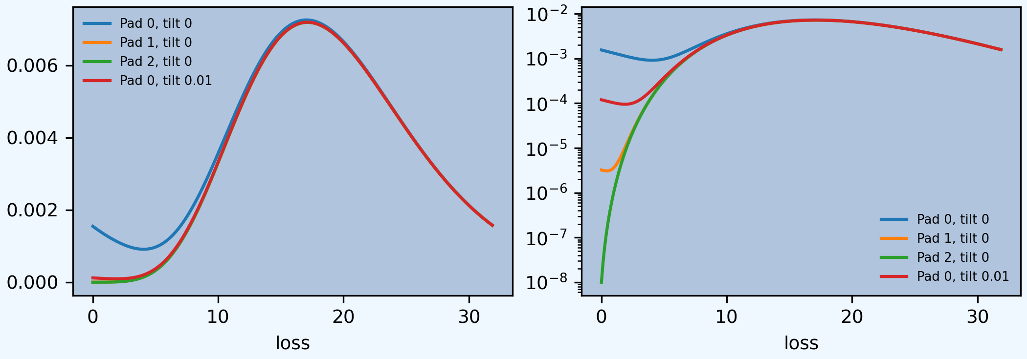
The next figure (compare Figure 1 in the paper, shown below) shows that padding, as recommended in Wang [1998], removes aliasing as effectively as padding, albeit at the expense of a longer FFT computation. The log density shows the aliasing is completely removed.
In [20]: f, axs = plt.subplots(1, 2, figsize=(2 * 3.5, 2.45), constrained_layout=True, squeeze=True)

In [21]: ax0, ax1 = axs.flat

In [22]: df.plot(ax=ax0, logy=False)
Out[22]: <Axes: xlabel='loss'>

In [23]: df.plot(ax=ax1, logy=True)
Out[23]: <Axes: xlabel='loss'>

In [24]: ax0.legend(loc='upper left')
Out[24]: <matplotlib.legend.Legend at 0x7f1b75ce6020>

In [25]: ax1.legend(loc='lower right');

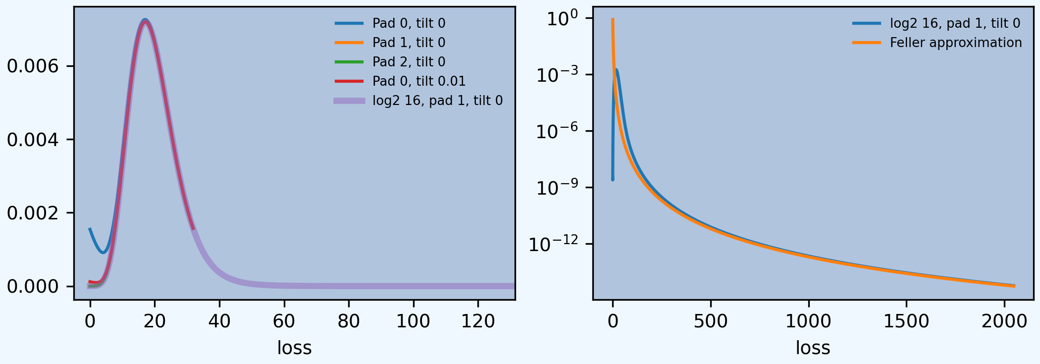
Clearly there is not enough space with only 2**8 buckets. Expanding to 2**16 and using a finer bucket covers a more realistic range. The log density plot shows a change in regime from Poisson body to Pareto tail. The extreme tail can be approximated by differentiating Feller’s theorem, which says the survival function is converges to \(20\mathsf{Pr}(X>x)\) where \(X\) is the Pareto severity (right hand plot). The multiplication by four accounts for the different bs values.
In [26]: f, axs = plt.subplots(1, 2, figsize=(2 * 3.5, 2.45), constrained_layout=True, squeeze=True)

In [27]: ax0, ax1 = axs.flat

In [28]: df.plot(ax=ax0, logy=False)
Out[28]: <Axes: xlabel='loss'>

In [29]: (bit * 4).plot(ax=ax0, lw=3, alpha=.5);

In [30]: bit.plot(ax=ax1, logy=True);

# density from tail, need to divide by bs
In [31]: ax1.plot(bit.index, (20*4/3*a.bs)*(3/(3+bit.index))**5, label='Feller approximation');

In [32]: ax0.set(xlim=[-5, a.q(0.99999)]);

In [33]: ax0.legend(loc='upper right');

In [34]: ax1.legend(loc='upper right');
2.13.2.2. Choice of Bandwidth (Bucket Size)
This example replicates parts of Table 1. As well as the 99.9%ile it shows the 99.9999%ile.
In [35]: import pandas as pd

In [36]: a = build('agg EF.2 50 claims sev expon poisson', update=False)

In [37]: ans = []

In [38]: for log2, bs in zip([10, 10, 10, 16, 16, 16, 16], [1, 1/2, 1/8, 1/8, 1/16, 1/64, 1/512]):
   ....:     a.update(log2=log2, bs=bs, padding=1)
   ....:     ans.append([log2, 1/bs, a.q(0.999), a.q(1-1e-6)])
   ....:

In [39]: df = pd.DataFrame(ans, columns=['log2', '1/bs', 'p999', 'p999999'])

In [40]: qd(df, accuracy=4)

   log2  1/bs   p999  p999999
0    10     1     84      107
1    10     2   84.5      108
2    10     8 85.125   108.25
3    16     8 85.125   108.25
4    16    16 85.125   108.25
5    16    64 85.109   108.23
6    16   512 85.105   108.23