2.13.3. Denuit (2019 and 2022)
2.13.3.1. Poisson/Discrete Example (6.1)
Example from Denuit [2019], Size-biased transform and conditional mean risk sharing, with application to p2p insurance and tontines.
In [1]: from aggregate import build, qd

In [2]: p = build('''
   ...: port Denuit6.1
   ...:     agg P1 0.08 claims dsev [1 2 3 4] [.1  .2  .4 .3] poisson
   ...:     agg P2 0.08 claims dsev [1 2 3 4] [.15 .25 .3 .3] poisson
   ...:     agg P3 0.10 claims dsev [1 2 3 4] [.1  .2  .4 .3] poisson
   ...:     agg P4 0.10 claims dsev [1 2 3 4] [.15 .25 .3 .3] poisson
   ...: ''', bs=1, log2=10)
   ...:

In [3]: qd(p)

            E[X] Est E[X]    Err E[X]   CV(X) Est CV(X)  Skew(X) Est Skew(X)
unit  X
P1    Freq  0.08                       3.5355             3.5355
      Sev    2.9      2.9 -1.1102e-16 0.32531   0.32531 -0.51452    -0.51452
      Agg  0.232    0.232  4.0856e-13  3.7179    3.7179   3.9518      3.9518
P2    Freq  0.08                       3.5355             3.5355
      Sev   2.75     2.75           0 0.37921   0.37921 -0.28106    -0.28106
      Agg   0.22     0.22  3.7326e-13  3.7812    3.7812   4.0928      4.0928
P3    Freq   0.1                       3.1623             3.1623
      Sev    2.9      2.9 -1.1102e-16 0.32531   0.32531 -0.51452    -0.51452
      Agg   0.29     0.29 -4.5741e-14  3.3254    3.3254   3.5346      3.5346
P4    Freq   0.1                       3.1623             3.1623
      Sev   2.75     2.75           0 0.37921   0.37921 -0.28106    -0.28106
      Agg  0.275    0.275  1.1036e-13   3.382     3.382   3.6607      3.6607
total Freq  0.36                       1.6667             1.6667
      Sev  2.825    2.825 -3.3307e-16 0.35299           -0.40097
      Agg  1.017    1.017 -5.6621e-15  1.7675    1.7675   1.8952      1.8952
log2 = 10, bandwidth = 1, validation: fails agg mean error >> sev, possible aliasing; try larger bs.
Computation of \(\mathsf{E}[X_i\mid X=x]\) and \(\mathsf{E}[X_i\mid X=x]/x\) as a function of \(x\).
The first function, called \(\kappa_i(x)\) in PIR, is computed automatically by the portfolio class as
exeqa_line (expectation given \(X\) equals \(x\)). The original figure is shown below.
In [4]: bit = p.density_df.query('p_total > 0').iloc[1:]

In [5]: rat = bit.filter(regex='exeqa_P').apply(
   ...:     lambda x: x / bit.loss.to_numpy(), axis=0)
   ...:

In [6]: ax = rat.plot.bar(ylim=[-0.05,1.05], stacked=True, figsize=(3.5, 2.45))

In [7]: ax.set(xlim=[-0.5, 15.5], ylim=[0,1]);

In [8]: ax.legend().set(visible=False);
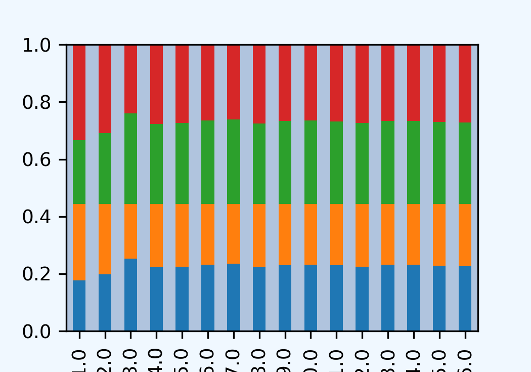
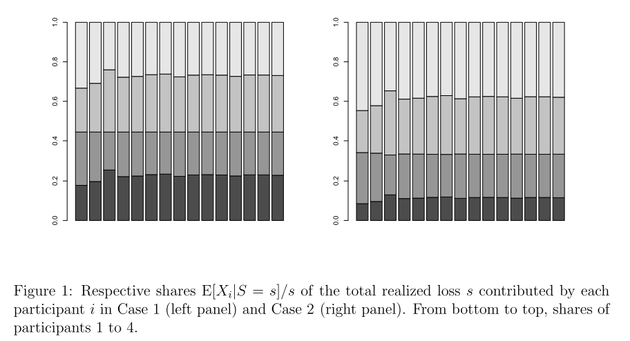
All the values are available as a table. These are consistent with numbers mentioned in the text.
In [9]: from pandas import option_context

In [10]: b = bit.filter(regex='exeqa_P').apply(
   ....:     lambda x: x / bit.loss.to_numpy(), axis=0)
   ....:

In [11]: b.index = b.index.astype(int)

In [12]: b.index.name = 'a'

In [13]: qd(b)

    exeqa_P1  exeqa_P2  exeqa_P3  exeqa_P4
a
1    0.17778   0.26667   0.22222   0.33333
2    0.19729   0.24716   0.24661   0.30895
3    0.25219   0.19226   0.31523   0.24032
4    0.22212   0.22232   0.27765    0.2779
5    0.22524   0.21921   0.28155   0.27401
6    0.23238   0.21207   0.29047   0.26508
7    0.23486   0.20958   0.29358   0.26198
8    0.22365    0.2208   0.27956     0.276
9    0.23064    0.2138   0.28831   0.26725
10   0.23224    0.2122    0.2903   0.26526
11   0.23056   0.21388    0.2882   0.26735
12   0.22551   0.21893   0.28189   0.27366
..       ...       ...       ...       ...
30   0.22858   0.21586   0.28573   0.26982
31   0.22829   0.21615   0.28537   0.27017
32   0.22872   0.21571    0.2859   0.26963
33   0.22893   0.21549   0.28617   0.26937
34   0.22839     0.216   0.28551   0.26999
35   0.22829    0.2161   0.28537   0.27006
36   0.22865   0.21576   0.28577   0.26966
37   0.22863   0.21571   0.28579   0.26959
38   0.22816   0.21601   0.28522    0.2699
39   0.22816   0.21599   0.28513   0.26976
40   0.22849   0.21582   0.28545   0.26962
41   0.22806   0.21556   0.28498    0.2692
Proportion of expected loss by unit.
In [14]: bb = p.describe.xs('Agg', axis=0, level=1)[['E[X]']]

In [15]: qd(bb / bb.iloc[-1,0])

         E[X]
unit
P1    0.22812
P2    0.21632
P3    0.28515
P4     0.2704
total       1
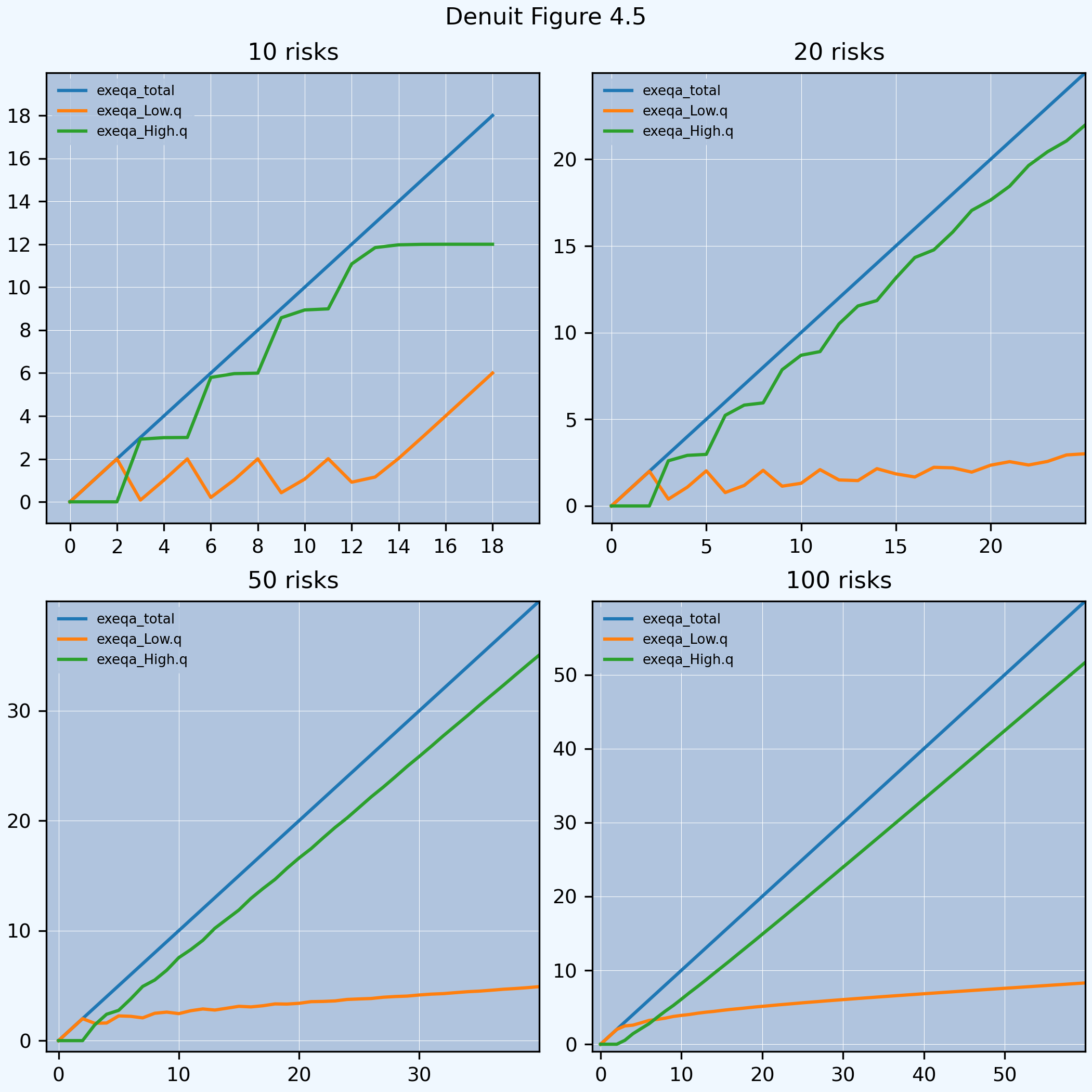
2.13.3.2. Mortality Example and Figure
Example from Denuit et al. [2022], Mortality Credits with Large Survivor Funds. Reproducing Figure 4.5.
In [16]: import matplotlib.pyplot as plt; import pandas as pd

In [17]: wl = 0.6; wh = 1 - wl; ql = .1; qh = .2; al = 1; ah = 3

In [18]: ports = {}

In [19]: for n in (10, 20, 50, 100):
   ....:     ports[n] = build(f'port DR.4.3 '
   ....:           f'agg Low.q  {wl * n * ql} claims dsev [{al}] binomial {ql}'
   ....:           f'agg High.q {wh * n * qh} claims dsev [{ah}] binomial {qh}'
   ....:          , bs=1, log2=8)
   ....:

In [20]: audit = pd.concat([i.describe for i in ports.values()], keys=ports.keys(), names=['n', 'unit', 'X'])

In [21]: qd(audit.xs('Agg', axis=0, level=2)['E[X]'].unstack(1))

unit  Low.q  High.q  total
n
10      0.6     2.4      3
20      1.2     4.8      6
50        3      12     15
100       6      24     30

In [22]: fig, axs = plt.subplots(2, 2, figsize=(2 * 3.5, 2 * 3.5), constrained_layout=True, squeeze=True)

In [23]: for ax, (n, port), mx, t in zip(axs.flat, ports.items(), [20, 25, 40, 60], [2, 5, 10, 10]):
   ....:     lm = [-1, mx]
   ....:     port.density_df.query('p_total > 0').filter(regex='exeqa_[LHt]').plot(ax=ax, xlim=lm, ylim=lm)
   ....:     ax.set_xticks(range(0, mx, t))
   ....:     ax.set_yticks(range(0, mx, t))
   ....:     ax.grid(lw=.25, c='w')
   ....:     ax.set(title=f'{n} risks')
   ....:

In [24]: fig.suptitle('Denuit Figure 4.5')
Out[24]: Text(0.5, 0.98, 'Denuit Figure 4.5')