2.13.7. Enterprise Risk Analysis
This section re-analyzes reinsurance structure alternatives introduced in Brehm et al. [2007], Enterprise Risk Analysis for Property & Liability Insurance Companies. This book is the ERM text on the syllabus for CAS Exam Part 7.
2.13.7.1. Reinsurance Example
This section analyzes the example given in Section 2.5 of Enterprise Risk Analysis.
Assumptions. ABCD writes 33M excess property and casualty business.
ABCD total gross
Loss ratio: 69.36%
Expense ratio: 23%
Combined ratio: 92.36%
Margin 2.52M
Casualty
14M premium
78% expected loss ratio
5M limits
4M xs 1M reinsurance, ceded premium 4.41M
Property
19M premium
63% expected loss ratio
20M limits
17M xs 3M per risk reinsurance, ceded premium 2.36M
95% share of 24M xs 1M cat reinsurance, ceded premium 1.53M with 1@100%
Cat program designed to cover to 250-year event.
Reinsurance total
Average recoveries 5.08M
Ceded premium 8.3M
Net premium 24.7M
Mythical alternative program
Stop-loss, 20 xs 30, ceded premium 1.98
Additional assumptions. There are no details of the stochastic model, so we assume
Frequency and severity models per DecL below,
Split the property losses into cat and non-cat by assuming that cat premium equals 2M, non-cat premium 17M, at the same loss ratios (this is just a split of losses, the by line loss ratios are not used), and
Cat, non-cat and casualty are independent.
Free and unlimited reinstatements on the catastrophe protection. See REF for a discussion of reinstatements.
2.13.7.2. Stochastic Models and Baseline Analysis
Construct the gross and net portfolios. All amounts in millions.
2.13.7.2.1. Gross Portfolio
The 250-year cat PML is printed last, to compare with the 25M program.
In [1]: from aggregate import build, qd, mv

In [2]: import pandas as pd

In [3]: import matplotlib.pyplot as plt

In [4]: abcd = build('port ABCD '
   ...:          'agg Casualty 14.0 premium at 78% lr '
   ...:              '5 xs 0 '
   ...:              'sev lognorm 0.1 cv 10 '
   ...:              'mixed gamma 0.3 '
   ...:          'agg PropertyNC 17.0 premium at 63% lr '
   ...:              '25 xs 0 '
   ...:              'sev lognorm [0.1 1] cv [5 10] wts [.7 .3] '
   ...:              'mixed gamma 0.1 '
   ...:          'agg PropertyC 2.0 premium at 63% lr '
   ...:              '150 xs 0 '
   ...:              'sev 3 * pareto 2.375 - 3 '
   ...:              'poisson ', bs=1/128, approximation='exact')
   ...:

In [5]: qd(abcd)

                    E[X] Est E[X]    Err E[X]   CV(X) Est CV(X)  Skew(X) Est Skew(X)
unit       X
Casualty   Freq   125.93                      0.31296            0.60054
           Sev  0.086717 0.086436  -0.0032438  4.0147    4.0286   9.5592      9.5552
           Agg     10.92   10.885  -0.0032438 0.47532   0.47626  0.88481     0.88565
PropertyNC Freq   34.918                      0.19657            0.24744
           Sev   0.30672  0.30659 -0.00041535    4.91    4.9121   11.569      11.569
           Agg     10.71   10.706 -0.00041535 0.85384   0.85419   1.9358      1.9358
PropertyC  Freq   0.5801                       1.3129             1.3129
           Sev     2.172    2.172 -9.2692e-07  2.0207    2.0207   11.511      11.511
           Agg      1.26     1.26 -9.2692e-07  2.9601    2.9601   12.398      12.398
total      Freq   161.42                      0.24785            0.57516
           Sev    0.1418  0.14155  -0.0017419  5.8043             23.386
           Agg     22.89    22.85  -0.0017419 0.48741   0.48813   1.6182      1.6193
log2 = 16, bandwidth = 1/128, validation: fails sev mean, agg mean.

In [6]: mv(abcd)
mean     = 22.89
variance = 124.4768
std dev  = 11.1569

In [7]: print(abcd['PropertyC'].q(0.996))
22.859375
2.13.7.2.2. Net Portfolio
In [8]: abcd_net = build('port ABCD:Net '
   ...:          'agg Casualty 14.0 premium at 78% lr '
   ...:              '5 xs 0 '
   ...:              'sev lognorm 0.1 cv 10 '
   ...:              'occurrence net of 4 xs 1 '
   ...:              'mixed gamma 0.3 '
   ...:          'agg PropertyNC 17.0 premium at 63% lr '
   ...:              '25 xs 0 '
   ...:              'sev lognorm [0.1 1] cv [5 10] wts [.7 .3] '
   ...:              'occurrence net of 17 xs 3 '
   ...:              'mixed gamma 0.1 '
   ...:          'agg PropertyC 2.0 premium at 63% lr '
   ...:              '150 xs 0 '
   ...:              'sev 3 * pareto 2.375 - 3 '
   ...:              'occurrence net of 24 xs 1 '
   ...:              'poisson ', bs=1/128, approximation='exact')
   ...:

In [9]: qd(abcd_net)

                    E[X] Est E[X] Err E[X]   CV(X) Est CV(X)  Skew(X) Est Skew(X)
unit       X
Casualty   Freq   125.93                   0.31296            0.60054
           Sev  0.086717 0.065564 -0.24393  4.0147    2.5318   9.5592      4.1714
           Agg     10.92   8.2563 -0.24393 0.47532    0.3858  0.88481     0.65534
PropertyNC Freq   34.918                   0.19657            0.24744
           Sev   0.30672   0.2098 -0.31597    4.91    2.8604   11.569      6.1847
           Agg     10.71   7.3259 -0.31597 0.85384   0.52244   1.9358      1.0361
PropertyC  Freq   0.5801                    1.3129             1.3129
           Sev     2.172  0.80417 -0.62976  2.0207    2.7345   11.511      36.228
           Agg      1.26   0.4665 -0.62976  2.9601    3.8228   12.398      40.649
total      Freq   161.42                   0.24785            0.57516
           Sev    0.1418 0.099419 -0.29888  5.8043             23.386
           Agg     22.89   16.049 -0.29888 0.48741   0.32957   1.6182      2.0938
log2 = 16, bandwidth = 1/128, validation: n/a, reinsurance.

In [10]: qd(abcd_net.est_sd)
5.2892
2.13.7.2.3. Ceded Portfolio
In [11]: abcd_ceded = build('port ABCD:Ceded '
   ....:          'agg Casualty 14.0 premium at 78% lr '
   ....:              '5 xs 0 '
   ....:              'sev lognorm 0.1 cv 10 '
   ....:              'occurrence ceded to 4 xs 1 '
   ....:              'mixed gamma 0.3 '
   ....:          'agg PropertyNC 17.0 premium at 63% lr '
   ....:              '25 xs 0 '
   ....:              'sev lognorm [0.1 1] cv [5 10] wts [.7 .3] '
   ....:              'occurrence ceded to 17 xs 3 '
   ....:              'mixed gamma 0.1 '
   ....:          'agg PropertyC 2.0 premium at 63% lr '
   ....:              '150 xs 0 '
   ....:              'sev 3 * pareto 2.375 - 3 '
   ....:              'occurrence ceded to 24 xs 1 '
   ....:              'poisson ', bs=1/128, approximation='exact')
   ....:

In [12]: qd(abcd_ceded)

                    E[X] Est E[X] Err E[X]   CV(X) Est CV(X)  Skew(X) Est Skew(X)
unit       X
Casualty   Freq   125.93                   0.31296            0.60054
           Sev  0.086717 0.020872 -0.75931  4.0147    11.205   9.5592      14.019
           Agg     10.92   2.6283 -0.75931 0.47532    1.0464  0.88481      1.3572
PropertyNC Freq   34.918                   0.19657            0.24744
           Sev   0.30672 0.096787 -0.68444    4.91    10.657   11.569       13.51
           Agg     10.71   3.3796 -0.68444 0.85384    1.8142   1.9358      2.3095
PropertyC  Freq   0.5801                    1.3129             1.3129
           Sev     2.172   1.3679 -0.37024  2.0207     2.254   11.511      4.2512
           Agg      1.26   0.7935 -0.37024  2.9601    3.2375   12.398      5.6851
total      Freq   161.42                   0.24785            0.57516
           Sev    0.1418 0.042134 -0.70286  5.8043             23.386
           Agg     22.89   6.8014 -0.70286 0.48741    1.0577   1.6182      1.7643
log2 = 16, bandwidth = 1/128, validation: n/a, reinsurance.

In [13]: qd(abcd_ceded.est_sd)
7.1941
2.13.7.2.4. Reinsurance Summary
The bottom table shows expected losses, counts, severity, loss ratios and margins implicit in the given reinsurance structure, pricing, and the gross stochastic model. The non-cat property reinsurance has the highest ceded loss ratio and the cat program the lowest.
In [14]: re_all = pd.concat((a.reinsurance_occ_layer_df for a in abcd_net),
   ....:     keys=abcd_net.unit_names, names=['unit', 'share', 'limit', 'attach']); \
   ....: re_all = re_all.drop('gup', axis=0, level=3); \
   ....: qd(re_all, sparsify=False)
   ....:

stat                              ex     ex      ex     cv     cv      cv      en severity     pct
view                           ceded    net subject  ceded    net subject   ceded    ceded   ceded
unit       share limit attach
Casualty   1.0   4.0   1.0    2.6283 8.2563  10.885 11.205 2.5318  4.0286   2.007   1.3096 0.24147
PropertyNC 1.0   17.0  3.0    3.3796 7.3259  10.706 10.657 2.8604  4.9121 0.65611    5.151 0.31569
PropertyC  1.0   24.0  1.0    0.7935 0.4665    1.26  2.254 2.7345  2.0207 0.29294   2.7088 0.62976

In [15]: re_summary = re_all.iloc[:, [0, 3, 6, 7]]; \
   ....: re_summary.columns = ['ex', 'cv', 'en', 'severity']; \
   ....: re_summary['premium'] = [4.41, 2.36, 1.53]; \
   ....: re_summary['lr'] = re_summary.ex / re_summary.premium; \
   ....: re_summary['margin'] = re_summary.premium - re_summary.ex; \
   ....: qd(re_summary)
   ....:

                                  ex     cv      en  severity  premium      lr  margin
unit       share limit attach
Casualty   1.0   4.0   1.0    2.6283 11.205   2.007    1.3096     4.41 0.59599  1.7817
PropertyNC 1.0   17.0  3.0    3.3796 10.657 0.65611     5.151     2.36   1.432 -1.0196
PropertyC  1.0   24.0  1.0    0.7935  2.254 0.29294    2.7088     1.53 0.51863  0.7365
2.13.7.2.5. Underwriting Result Distributions
Make the underwriting result distributions, including the proposed stop loss reinsurance (computed by hand).
The dataframe compare accumulates the gross, ceded, and net probability mass functions. We use these
to determine statistics and to plot.
In [16]: compare = abcd.density_df[['loss', 'p_total']]; \
   ....: compare.columns = ['loss', 'gross']; \
   ....: compare['gross_uw'] = 33 - compare.loss; \
   ....: compare['net_current'] = abcd_net.density_df.p_total; \
   ....: compare['net_current_uw'] = 33 - 4.41 - 2.36 - 1.53 - compare.loss;
   ....:

In [17]: from aggregate import make_ceder_netter

In [18]: compare['net_stoploss'] = abcd.density_df.p_total; \
   ....: c, n = make_ceder_netter([(1, 20, 30)]); \
   ....: compare['nsll'] = n(compare.loss); \
   ....: g = compare.groupby('nsll').net_stoploss.sum(); \
   ....: compare['net_stoploss'] = 0.0; \
   ....: compare.loc[g.index, 'net_stoploss'] = g; \
   ....: compare['net_stoploss_uw'] = 33 - 1.98 - compare.loss;
   ....:
2.13.7.2.6. Comparison with ERA Book Figures
Statistics summary, compare Figure 2.5.2.
In [19]: from aggregate import MomentWrangler

In [20]: from scipy.interpolate import interp1d

In [21]: ans = []; cdfs = []

In [22]: for xs, den in [(compare.gross_uw, compare.gross), (compare.net_current_uw, compare.net_current),
   ....:                  (compare.net_stoploss_uw, compare.net_stoploss)]:
   ....:     xd = xs * den
   ....:     ex1 = np.sum(xd)
   ....:     xd *= xs
   ....:     ex2 = np.sum(xd)
   ....:     ex3 = np.sum(xd * xs)
   ....:     mw = MomentWrangler()
   ....:     mw.noncentral = ex1, ex2, ex3
   ....:     ans.append(mw)
   ....:     cdfs.append(interp1d(den.cumsum(), xs))
   ....:

In [23]: fig_252 = pd.concat([i.stats for i in ans], keys=['Gross', 'Current', 'StopLoss'], axis=1)

In [24]: for p in [0.01, 0.99]:
   ....:     fig_252.loc[f'q({p})'] = [float(i(p)) for i in cdfs]
   ....:

In [25]: qd(fig_252)

          Gross  Current  StopLoss
ex        10.15   8.6513    10.021
var      124.41   27.975    58.777
sd       11.154   5.2892    7.6666
cv       1.0989  0.61137   0.76502
skew    -1.6193  -2.0938   -1.0088
q(0.01)   25.98   18.081        24
q(0.99)  -25.76  -5.6036   -7.7399
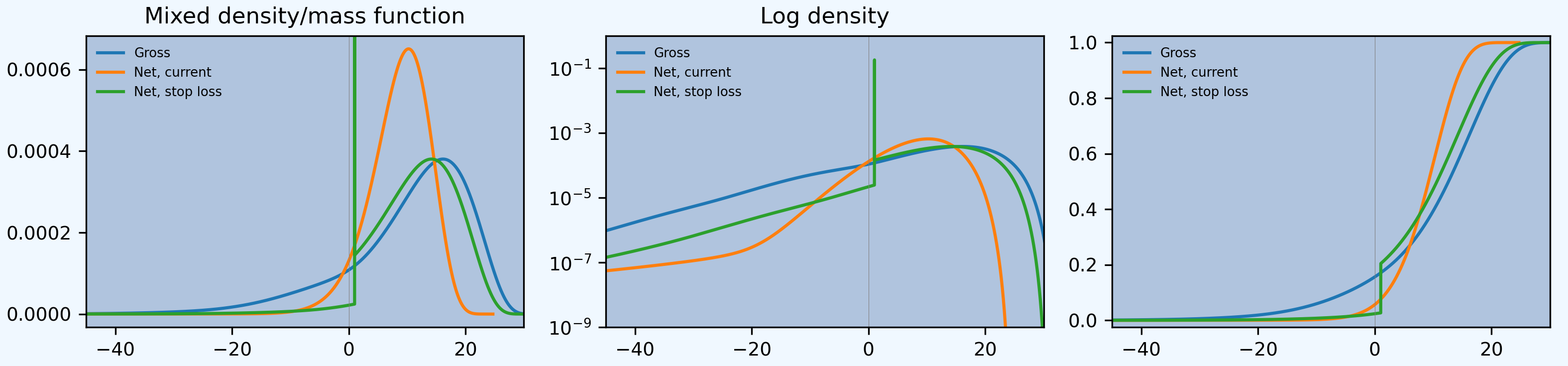
Plot of densities and distributions, compare Figure 2.5.3 and 2.5.4.
In [26]: fig, axs = plt.subplots(1, 3, figsize=(3 * 3.5, 2.45), constrained_layout=True)

In [27]: ax0, ax1, ax2 = axs.flat

In [28]: for ax in [ax0, ax1]:
   ....:     ax.plot(compare.gross_uw, compare.gross, label='Gross')
   ....:     ax.plot(compare.net_current_uw, compare.net_current, label='Net, current')
   ....:     yl = ax.get_ylim()
   ....:     ax.plot(compare.net_stoploss_uw, compare.net_stoploss, label='Net, stop loss')
   ....:     ax.legend(loc='upper left')
   ....:     ax.set(xlim=[-45, 30], ylim=yl)
   ....:     ax.axvline(0, lw=.25, c='C7')
   ....:

In [29]: ax1.set(yscale='log', ylim=[1e-9, 1], title='Log density'); \
   ....: ax0.set(title='Mixed density/mass function');
   ....:

In [30]: ax2.plot(compare.gross_uw, 1 - compare.gross.cumsum(), label='Gross'); \
   ....: ax2.plot(compare.net_current_uw, 1 - compare.net_current.cumsum(), label='Net, current'); \
   ....: ax2.plot(compare.net_stoploss_uw, 1 - compare.net_stoploss.cumsum(), label='Net, stop loss'); \
   ....: ax2.legend(loc='upper left'); \
   ....: ax2.set(xlim=[-45, 30], ylim=[-0.025, 1.025]);
   ....:

In [31]: ax2.axvline(0, lw=.25, c='C7');
Numerical distribution of underwriting results at various return points, compare Figure 2.5.5. Given there was no information about the stochastic model provided, and the model here is based on common benchmarks, the agreement between the two distributions is striking.
In [32]: fig_255 = pd.DataFrame(columns=['Gross', 'Current', 'StopLoss'], dtype=float)

In [33]: for p in [.0025, .005, 0.0075, .01, .0125, .015, .0175, .02,
   ....:           .04, .06, .08, .1, .12, .14, .16, .18, .2, .22, .24,
   ....:           .25, .26, .28, .3, .32, .34, .36, .38, .4, .42, .44,
   ....:           .46, .48, .5]:
   ....:     fig_255.loc[p] = [float(i(1-p)) for i in cdfs]
   ....:

In [34]: fig_255.index.name = 'p'

In [35]: qd(fig_255, float_format=lambda x: f'{x:.3f}', max_rows=len(fig_255))

         Gross  Current  StopLoss
p
0.0025 -38.503  -10.257   -20.483
0.0050 -32.113   -7.826   -14.093
0.0075 -28.394   -6.514   -10.374
0.0100 -25.760   -5.604    -7.740
0.0125 -23.740   -4.902    -5.720
0.0150 -22.114   -4.328    -4.094
0.0175 -20.758   -3.842    -2.738
0.0200 -19.595   -3.420    -1.575
0.0400 -13.603   -1.182     1.021
0.0600  -9.962    0.182     1.021
0.0800  -7.211    1.186     1.022
0.1000  -4.936    1.991     1.023
0.1200  -2.978    2.669     1.024
0.1400  -1.263    3.259     1.025
0.1600   0.246    3.784     1.026
0.1800   1.575    4.259     1.027
0.2000   2.752    4.695     1.028
0.2200   3.801    5.100     1.821
0.2400   4.745    5.478     2.765
0.2500   5.183    5.659     3.203
0.2600   5.603    5.835     3.623
0.2800   6.391    6.173     4.411
0.3000   7.121    6.496     5.141
0.3200   7.802    6.805     5.822
0.3400   8.442    7.103     6.462
0.3600   9.047    7.390     7.067
0.3800   9.622    7.669     7.642
0.4000  10.171    7.941     8.191
0.4200  10.697    8.206     8.717
0.4400  11.203    8.465     9.223
0.4600  11.692    8.720     9.712
0.4800  12.167    8.970    10.187
0.5000  12.628    9.217    10.648
2.13.7.3. Modern Analysis
The first step is to analyze the pricing in the context of needed capital. Strip expenses out (at 23% across all units) to determine a net (of expenses) technical premium.
In [36]: er = 0.23

In [37]: df = pd.DataFrame({'unit': ['Casualty', 'PropertyNC', 'PropertyC'],
   ....:                           'prem': [14, 17, 2],
   ....:                             'gross_loss': [a.est_m for a in abcd]}).set_index('unit')
   ....:

In [38]: df['ceded_prem'] = [4.41, 2.36, 1.53]; \
   ....: df['net_prem'] = df.prem - df.ceded_prem; \
   ....: df['tech_prem'] = df.prem * (1 - er); \
   ....: df['margin'] = df.tech_prem - df.gross_loss; \
   ....: df.loc['Total'] = df.sum(0); \
   ....: df['lr'] = df.gross_loss / df.prem; \
   ....: df['cr'] = df.lr + er; \
   ....: df['tech_lr'] = df.gross_loss / df.tech_prem;
   ....:

In [39]: fp = lambda x: f'{x:.1%}';

In [40]: fc = lambda x: f'{x:.2f}'

In [41]: qd(df, float_format=fc, formatters={'lr':fp, 'cr': fp, 'tech_lr': fp})

            prem  gross_loss  ceded_prem  net_prem  tech_prem  margin    lr     cr tech_lr
unit
Casualty   14.00       10.88        4.41      9.59      10.78   -0.10 77.7% 100.7%  101.0%
PropertyNC 17.00       10.71        2.36     14.64      13.09    2.38 63.0%  86.0%   81.8%
PropertyC   2.00        1.26        1.53      0.47       1.54    0.28 63.0%  86.0%   81.8%
Total      33.00       22.85        8.30     24.70      25.41    2.56 69.2%  92.2%   89.9%
The example does not specify a capital standard. Let’s investigate the implied
return on capital at different capital standards. The capital standard is
expressed as a loss percentile. The next calculation produces a table of
returns expressed as a cost of capital (coc). It also shows the expected
policyholder deficit.
In [42]: tech_prem = df.loc['Total', 'tech_prem']; \
   ....: ps = [.99, .995, .996, .999]; \
   ....: As = [abcd.q(p) for  p in ps]; \
   ....: el = abcd.density_df.loc[As, 'exa_total']; \
   ....: margin = tech_prem - el; \
   ....: cocs = margin /  (As - tech_prem); \
   ....: summary = pd.DataFrame({'p': ps, 'a': As, 'prem':tech_prem, 'el': el,
   ....:                         'margin': margin, 'tech_lr': el / tech_prem, 'coc': cocs,
   ....:                        'epd': (abcd.est_m - el) / abcd.est_m}).set_index('p')
   ....:

In [43]: summary.index = [fp(i) for i in summary.index]; \
   ....: summary.index.name = 'p'; \
   ....: qd(summary, float_format=fc, formatters={'coc': fp, 'tech_lr': fp, 'epd': fp})
   ....:

          a  prem    el  margin tech_lr  coc  epd
p
99.0% 58.77 25.41 22.75    2.66   89.5% 8.0% 0.5%
99.5% 65.12 25.41 22.79    2.62   89.7% 6.6% 0.3%
99.6% 67.16 25.41 22.80    2.61   89.7% 6.2% 0.2%
99.9% 80.90 25.41 22.83    2.58   89.8% 4.6% 0.1%
Based on this analysis, we assume a 99.5% (200-year) capital standard, which gives a reasonable 8% return on capital. 200-year capital is also the Solvency II standard.
From here, the analysis could proceed in many directions. The approach we select is
Calibrate a set of distortions to total pricing on a gross basis with the 200-year capital standard.
Analyze the pricing implied by these distortions on the net book and its natural allocation by unit.
Compare the model value (implied ceded premium) with market reinsurance price.
The model value is the maximum amount that is consistent with pricing according to each distortion. Reinsurance cheaper than the model value is efficient: replacing traditional capital with reinsurance capital lowers the economic cost of bearing risk.
2.13.7.3.1. Calibrate Distortions
Extract the exact cost of capital implied by given gross pricing.
In [44]: coc = summary.loc['99.5%', 'coc']

In [45]: print(coc)
0.06591531668710866
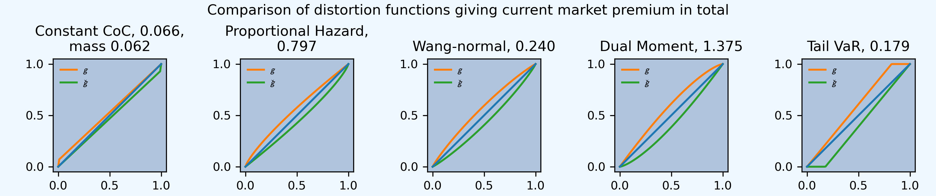
Calibrate distortions to current pricing. Use five one-parameter distortion families
constant cost of capital (CCoC),
proportional hazard (PH)
Wang,
dual, and
TVaR.
They are sorted from most tail-centric (expensive for tail risk) to cheapest. See Mildenhall and Major [2022].
The next dataframe shows the asset level and implied loss ratio,
distortion name, survival probability (0.5%), expected loss, premium, premium
to capital leverage (PQ), the cost of (return on) capital, the distortion
family parameter, and the parameterization error. The calibrated premium
matches the technical premium.
In [46]: abcd.calibrate_distortions(ROEs=[coc], Ps=[.995], strict='ordered');

In [47]: qd(abcd.distortion_df)

                                  S      L     P      PQ      Q      COC    param       error
a         LR       method
65.117188 0.896997 ccoc   0.0049978 22.793 25.41 0.63993 39.707 0.065915 0.065915           0
                   ph     0.0049978 22.793 25.41 0.63993 39.707 0.065915   0.7966  4.7227e-06
                   wang   0.0049978 22.793 25.41 0.63993 39.707 0.065915  0.24044  1.1474e-06
                   dual   0.0049978 22.793 25.41 0.63993 39.707 0.065915   1.3749 -7.4227e-11
                   tvar   0.0049978 22.793 25.41 0.63993 39.707 0.065915  0.17864  9.4873e-06
The plot show this effect: COC is fattest on the left for small exceedance probabilities (high losses), whereas TVaR is fattest on the right.
In [48]: fig, axs = plt.subplots(1, 5, figsize=(10.0, 2.1), constrained_layout=True)

In [49]: for ax, (k, v) in zip(axs.flat, abcd.dists.items()):
   ....:     v.plot(ax=ax)
   ....:

In [50]: fig.suptitle('Comparison of distortion functions giving current market premium in total')
Out[50]: Text(0.5, 0.98, 'Comparison of distortion functions giving current market premium in total')
2.13.7.3.2. Analyze Implied Pricing
Apply the distortions to the net portfolio and analyze the resulting pricing
using analyze_distortions(), which includes a by-unit margin
allocation. The dataframe ans.comp_df contains a wealth of other
information; we just focus on the premium. The last row, Technical, shows
market reinsurance pricing.
In [51]: abcd_net.dists = abcd.dists

In [52]: ansn = abcd_net.analyze_distortions(p=0.996, add_comps=False); \
   ....: ans = abcd.analyze_distortions(p=0.996, add_comps=False); \
   ....: bit = pd.concat((ans.comp_df.xs('P', 0, 1), ansn.comp_df.xs('P', 0, 1),
   ....:                 ans.comp_df.xs('P', 0, 1) - ansn.comp_df.xs('P', 0, 1)),
   ....:                 axis=1, keys=['gross', 'net', 'ceded']); \
   ....: bit = bit.iloc[[0, 2,-1, 1, -2]]; \
   ....: bit.loc['Technical'] = 0.0; \
   ....: bit.loc['Technical', 'gross'] = df.tech_prem.sort_index().values; \
   ....: bit.loc['Technical', 'ceded'] = df.ceded_prem.sort_index().values; \
   ....: bit.loc['Technical', 'net'] = df.net_prem.sort_index().values; \
   ....: qd(bit, sparsify=False, line_width=50)
   ....:

             gross     gross      gross  gross  \
line      Casualty PropertyC PropertyNC  total
Method
Dist ccoc   10.371    4.6237      10.55 25.545
Dist ph     11.347    1.5483     12.542 25.438
Dist wang   11.514    1.4754     12.439 25.428
Dist dual   11.698    1.4415     12.283 25.423
Dist tvar   11.908    1.4298     12.084 25.421
Technical    10.78      1.54      13.09  25.41

               net       net        net    net  \
line      Casualty PropertyC PropertyNC  total
Method
Dist ccoc   7.8043    2.3449     6.9327 17.082
Dist ph     8.6519   0.53481      7.977 17.164
Dist wang   8.7296   0.49483     8.0137 17.238
Dist dual   8.8065   0.47931     8.0416 17.327
Dist tvar   8.8941   0.47972     8.0693 17.443
Technical     9.59      0.47      14.64   24.7

             ceded     ceded      ceded  ceded
line      Casualty PropertyC PropertyNC  total
Method
Dist ccoc   2.5669    2.2788     3.6172 8.4632
Dist ph     2.6952    1.0135     4.5651 8.2738
Dist wang    2.784   0.98056     4.4253 8.1898
Dist dual   2.8917   0.96217     4.2413 8.0952
Dist tvar   3.0137   0.95009     4.0143 7.9781
Technical     4.41      1.53       2.36    8.3
2.13.7.3.3. Compare Model Value and Market Price
Focus on the last block above, under ceded. The rows Dist ... show the
model value of reinsurance according to each distortion. The row
Technical shows the market price. The market suggests to buy when the
value is greater than the price.
The analysis provides a clear answer only for casualty, where the model value of reinsurance is much lower than the market price for all distortions: don’t buy the reinsurance.
For property cat, CCoC, the most tail-centric distortion, sees a lot of value in the reinsurance — hardly surprising. All the other less tail-centric distortions do not see it as adding value overall (lower value than market price). The order of the distortions and their assessment of the value of cat reinsurance are perfectly aligned, as they were for casualty albeit in the opposite order.
For property non-cat, the PH and Wang distortions see value, the others do not, though dual is close. This is the most interesting case because the ranking does not agree with the distortion ordering (as it does for the other two units). Property non-cat contributes to volatility and tail-risk, and so is more nuanced. Management often struggles with property risk reinsurance because tail-centric measures understate the value it provides. Actuaries stuggle to find analytic methods that capture its management-perceived value. The range of distortions considered covers the two views well.
In total the program is not seen as good value by any of the distortions. Since they span the reasonable range of risk preferences, this is a robust result.
Management often cares about more than just tail risk and they generally rejects the findings from CCoC. Whether or not they see value in reinsurance is sensitive to their exact risk appetite. These findings are consistent with the fact that each company tends to structure its reinsurance differently, tailored to their own risk appetite. Difference in risk appetite have a material impact on decision making.
2.13.7.3.4. Analysis for Stop Loss Reinsurance
Here is the analysis for the stop loss reinsurance. This analysis is manual,
because the net of stop loss distribution for a Portfolio is not
currently built-in. We have to extract the relevant distributions and apply
the distortions, estimate a_stoploss the net asset requirement at
p=0.995 (rounded to be a multiple of bs), determine the net expected
loss and the model value. Recall compare.net_stoploss is the density of
the net of stop-loss loss outcome. S1 is used to create its survival
function, to which the distortion is applied to determine pricing. exa
and exag are the objective and risk adjusted losses (model value) given
an asset level a, computed as \(\int_0^a S\) and \(\int_0^a g
(S)\) respectively (see PIR REF). We then select the relevant row and assemble
the answer.
In [53]: S0 = pd.Series(compare.net_stoploss, index=compare.loss); \
   ....: S0.name = 'S'; \
   ....: S1 = S0[::-1].shift(1, fill_value=0).cumsum(); \
   ....: a0 = float(interp1d(S0.cumsum(), S0.index)(0.995)); \
   ....: a_stoploss = abcd.snap(a0); \
   ....: print(f'Net of stoploss assets {a_stoploss:.3f}');
   ....:
Net of stoploss assets 45.109

In [54]: net_el_stoploss_unlim = (compare.loss * compare.net_stoploss).sum(); \
   ....: net_el_stoploss = (np.minimum(compare.loss, a_stoploss) * compare.net_stoploss).sum(); \
   ....: epd = 1 - net_el_stoploss / net_el_stoploss_unlim; \
   ....: qd(pd.Series([net_el_stoploss_unlim, net_el_stoploss, epd], index=['unlimited net loss', 'net loss limited by assets', 'epd']));
   ....:

unlimited net loss              20.999
net loss limited by assets      20.941
epd                          0.0027373

In [55]: pricer = S1.to_frame().sort_index();

In [56]: for nm, dist in abcd.dists.items():
   ....:     pricer[f'{nm}_exa'] = pricer['S'].shift(1, fill_value=0).cumsum() * abcd.bs
   ....:     pricer[f'{nm}_gS'] = dist.g(pricer.S)
   ....:     pricer[f'{nm}_exag'] = pricer[f'{nm}_gS'].shift(1, fill_value=0).cumsum() * abcd.bs
   ....:     pricer = pricer.sort_index()
   ....:

In [57]: try:
   ....:     pricer = pricer.loc[[a_stoploss]]; \
   ....:     pricer.columns = pricer.columns.str.split('_', expand=True); \
   ....:     comp = pricer.stack(0).droplevel(0,0); \
   ....:     comp.loc['Technical'] = [net_el_stoploss, tech_prem - 1.98, np.nan]; \
   ....:     comp['stoploss_value'] = tech_prem - comp.exag; \
   ....:     comp = comp.sort_values('stoploss_value', ascending=False); \
   ....:     qd(comp)
   ....: except:
   ....:     print('Unspecfied error: TODO investigate.')
   ....:
Unspecfied error: TODO investigate.
The output table reveals that the stop loss value is greater than its market price for the CCoC, PH, and Wang distortions, but less for the dual and TVaR. Thus, management averse to tail risk regard it as beneficial, but those more concerned with volatility and body risk do not see it as worthwhile.
A note of caution is in order on this analysis. Stop loss structures are a broker favorite, but are generally not liked by reinsurers. Aggregate features are hard to underwrite and price, and the lower premium is not attractive. A treaty similar to the proposed stop loss would be very hard to find in the market.
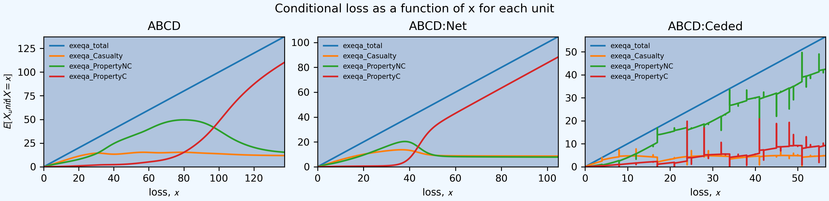
2.13.7.4. Visualizing Risk
The next figure shows the kappa functions, a handy way to visualize which units are contributing to total risk across the loss spectrum (see REF). Here the horizontal axis is total loss. The middle plot shows the reinsurance is quite effective at lowering the risk from Property NC (green line), but less effective at altering the risk profile of the other two lines. In particular, cat (red line) still dominates the tail risk.
In [58]: fig, axs = plt.subplots(1, 3, figsize=(3 * 3.5, 2.55), constrained_layout=True)

In [59]: for ax, a in zip(axs.flat, [abcd, abcd_net, abcd_ceded]):
   ....:     mx = a.q(0.9999)
   ....:     a.density_df.filter(regex='exeqa_[CPt]').plot(ax=ax,
   ....:         xlim=[0, mx], ylim=[0, mx], title=a.name);
   ....:     ax.set(xlabel='loss, $x$');
   ....:

In [60]: axs.flat[0].set(ylabel='$E[X_unit | X=x]$');

In [61]: fig.suptitle('Conditional loss as a function of x for each unit');