2.13.4. Loss Data Analytics Book
Examples from Jed Frees’ open source actuarial software. Text and github source available on-line.
2.13.4.1. Contents
2.13.4.2. Distribution Examples
2.13.4.2.1. Gamma distribution
In [1]: import scipy.stats as ss

In [2]: import numpy as np

In [3]: import matplotlib.pyplot as plt

In [4]: xs = np.linspace(0, 1000, 1001)

In [5]: fig, axs = plt.subplots(1, 2, figsize=(2 * 3.5, 2.45), constrained_layout=True, squeeze=True)

In [6]: ax0, ax1 = axs.flat

In [7]: for scale in [100, 150, 200, 250]:
   ...:     ax0.plot(xs, ss.gamma(2, scale=scale).pdf(xs), label=f'scale = {scale}')
   ...:

In [8]: for shape in [2, 3, 4, 5]:
   ...:     ax1.plot(xs, ss.gamma(shape, scale=100).pdf(xs), label=f'shape = {shape}')
   ...:

In [9]: for ax in axs.flat:
   ...:     ax.legend(loc='upper right')
   ...:     ax.set(ylabel='gamma density', xlabel='x')
   ...:

2.13.4.2.2. Pareto distribution
In [10]: xs = np.linspace(0, 3000, 3001)

In [11]: fig, axs = plt.subplots(1, 2, figsize=(2 * 3.5, 2.45), constrained_layout=True, squeeze=True)

In [12]: ax0, ax1 = axs.flat

In [13]: for scale in [2000, 2500, 3000, 3500]:
   ....:     ax0.plot(xs, ss.pareto(3, scale=scale, loc=-scale).pdf(xs), label=f'scale = {scale}')
   ....:

In [14]: for shape in [1,2,3,4]:
   ....:     ax1.plot(xs, ss.pareto(shape, scale=2000, loc=-2000).pdf(xs), label=f'shape = {shape}')
   ....:

In [15]: for ax in axs.flat:
   ....:     ax.legend(loc='upper right')
   ....:     ax.set(ylabel='Pareto density', xlabel='x')
   ....:

2.13.4.2.3. Weibull distribution
scipy.stats includes Weibull min (for positive \(x\)) and Weibull max (for negative \(x\)) distributions. We want the min version.
In [16]: xs = np.linspace(0, 400, 401)

In [17]: fig, axs = plt.subplots(1, 2, figsize=(2 * 3.5, 2.45), constrained_layout=True, squeeze=True)

In [18]: ax0, ax1 = axs.flat

In [19]: for scale in [50, 100, 150, 200]:
   ....:     ax0.plot(xs, ss.weibull_min(3, scale=scale).pdf(xs), label=f'scale = {scale}')
   ....:

In [20]: for shape in [1.5, 2, 2.5, 3]:
   ....:     ax1.plot(xs, ss.weibull_min(shape, scale=100).pdf(xs), label=f'shape = {shape}')
   ....:

In [21]: for ax in axs.flat:
   ....:     ax.legend(loc='upper right')
   ....:     ax.set(ylabel='Weibull_min density', xlabel='x')
   ....:

2.13.4.3. Mixture Example (3.3.5)
A collection of insurance policies consists of two types. 25% of policies are Type 1 and 75% of policies are Type 2. For a policy of Type 1, the loss amount per year follows an exponential distribution with mean 200, and for a policy of Type 2, the loss amount per year follows a Pareto distribution with parameters \(\alpha=3\) and \(\theta=200\). For a policy chosen at random from the entire collection of both types of policies, find the probability that the annual loss will be less than 100, and find the average loss.
Solution. The function pmv (print mean and variance) is a convenience.
In [22]: from aggregate import build, qd, mv

In [23]: def pmv(m, v):
   ....:     print(f'mean     = {m:.6g}\n'
   ....:           f'variance = {v:.7g}')
   ....:
Create the Aggregate object, display its describe dataframe and compare the cdf with the exact computation.
In [24]: a = build('agg lda.3.3.5 '
   ....:           '1 claim '
   ....:           'sev [200 200] * [expon pareto] [1 3] + [0 -200] wts [.25 .75] '
   ....:           'fixed',
   ....:           normalize=False)
   ....:

In [25]: qd(a)

      E[X] Est E[X]    Err E[X]  CV(X) Est CV(X) Skew(X) Est Skew(X)
X
Freq     1                           0
Sev    125      125 -2.3123e-05 1.4832    1.4754     inf      9.9477
Agg    125      125 -2.3123e-05 1.4832    1.4754     inf      9.9477
log2 = 16, bandwidth = 1/2, validation: fails sev cv, agg cv.

In [26]: a.sev.cdf(100), 0.25 * (1 - np.exp(-0.5)) + 0.75 * (1 - (2/3)**3)
Out[26]: (0.6261451128496194, 0.6261451128496194)
This example has a very thick tailed severity and it is best to specify normalized=False for the most accurate severity estimates. With default settings,
aggregate suffers considerable discretization error, with an estimated mean well below the actual 125. The sev.cdf method exposes the actual underlying
severity distribution cdf functions and reproduces the requested probability exactly. The object cdf function relies on the discretization and so is shifted by
half a bucket size. (Also available: sev.sf and sev.pdf.)
In [27]: a.cdf(100), a.sev.cdf(100 + a.bs/2)
Out[27]: (0.626889166181137, 0.6268891661811365)
2.13.4.4. Coverage Modifications
Deductible Example (3.4.1)
A claim severity distribution is exponential with mean 1000. An insurance company will pay the amount of each claim in excess of a deductible of 100. Calculate the variance of the amount paid by the insurance company for one claim, including the possibility that the amount paid is 0.
Solution. In this case we must use unconditional severity to include the possibility that the amount paid is 0. This is done by adding ! at the end of the severity specification. The moments are computed exactly without updating.
In [28]: import numpy as np

In [29]: a = build('agg lda.3.4.1 1 claim '
   ....:           'inf xs 100 sev 1000 * expon 1 ! '
   ....:           'fixed', update=False)
   ....:

In [30]: qd(a)

       E[X]  CV(X) Skew(X)
X
Freq      1      0
Sev  904.84 1.1002  2.0257
Agg  904.84 1.1002  2.0257
log2 = 0, bandwidth = na, validation: n/a, not updated.

In [31]: m = 1000 * np.exp(-0.1)

In [32]: mv(a)
mean     = 904.837
variance = 990944.1
std dev  = 995.462

In [33]: pmv(m, (2 * 1000**2 * np.exp(-0.1)) - m**2)
mean     = 904.837
variance = 990944.1
Deductible Example (3.4.2)
For an insurance:
Losses have a density function
\[\begin{split}f_{X}\left( x \right) = \left\{ \begin{matrix} 0.02x & 0 < x < 10, \\ 0 & \text{elsewhere.} \\ \end{matrix} \right.\end{split}\]The insurance has an ordinary deductible of 4 per loss.
\(Y^{P}\) is the claim payment per payment random variable.
Solution. The trick here is to realize that \(X\) is a beta variable with \(\alpha=2\) and \(\beta=1\).
In [34]: a = build('agg lda.3.4.2 1 claim 6 xs 4 sev 10 * beta 2 1 fixed')

In [35]: qd(a)

       E[X] Est E[X]   Err E[X]   CV(X) Est CV(X)  Skew(X) Est Skew(X)
X
Freq      1                           0
Sev  3.4286   3.4286 1.0348e-10 0.48947   0.48947 -0.29313    -0.29313
Agg  3.4286   3.4286 1.0348e-10 0.48947   0.48947 -0.29313    -0.29313
log2 = 16, bandwidth = 1/4096, validation: not unreasonable.

In [36]: mv(a)
mean     = 3.42857
variance = 2.816327
std dev  = 1.67819
Limit Example (3.4.4)
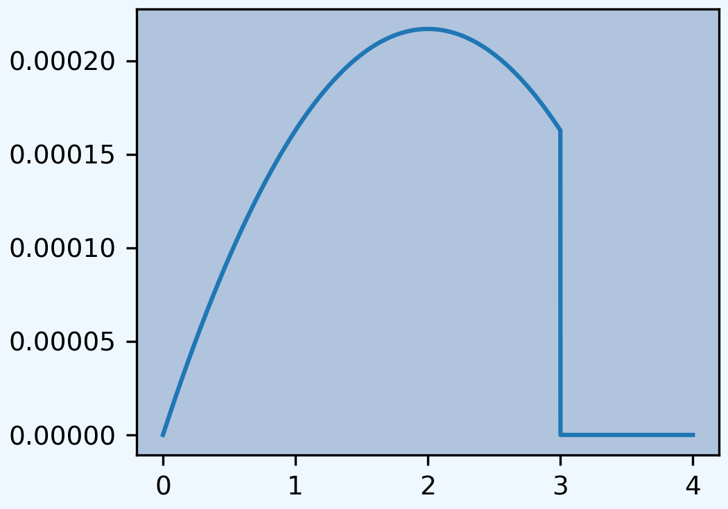
Under a group insurance policy, an insurer agrees to pay 100% of the medical bills incurred during the year by employees of a small company, up to a maximum total of one million dollars. The total amount of bills incurred, \(X\), has pdf
where \(x\) is measured in millions. Calculate the total amount, in millions of dollars, the insurer would expect to pay under this policy.
Solution. In this case the distribution has no obvious parametric form—though it is related to a beta. We can solve it in aggregate by using a custom empirical distribution.
In [37]: xs = np.linspace(0, 4, 2**13, endpoint=False)

In [38]: F = np.where(xs<3,(xs * xs  * (2 - xs / 3)) / 9, 1)

In [39]: ps = np.diff(F, append=1)

In [40]: fig, ax = plt.subplots(1, 1, figsize=(3.5, 2.45), constrained_layout=True, squeeze=True)

In [41]: ax.plot(xs, ps);
When the empirical distribution has many entries it is faster to build the Aggregate object directly, rather than use DecL. The moments of the severity and aggregate distribution are computed from the numerical approximation during creation. There is no need to update the object.
In [42]: from aggregate import Aggregate

In [43]: a = Aggregate('Example', exp_en=1, sev_name='dhistogram', sev_xs=xs, sev_ps=ps,
   ....:              exp_attachment=0, exp_limit=1, freq_name='fixed')
   ....:

In [44]: print(a)
aggregate object name    Example
claim count              1.00
frequency distribution   fixed
severity distribution    dhistogram, 1 xs 0.
        E[X]  CV(X)  Skew(X)
X
Freq       1      0      NaN
Sev  0.93514 0.1826  -2.9018
Agg  0.93514 0.1826  -2.9018
Limit and Deductible Example (3.4.5)
The ground up loss random variable for a health insurance policy in 2006 is modeled with \(X\), a random variable with an exponential distribution having mean 1000. An insurance policy pays the loss above an ordinary deductible of 100, with a maximum annual payment of 500. The ground up loss random variable is expected to be 5% larger in 2007, but the insurance in 2007 has the same deductible and maximum payment as in 2006. Find the percentage increase in the expected cost per payment from 2006 to 2007.
Solution. Trend increases the ground-up severity distribution but not the limit and attachment. The calculation is performed exactly on creation; again, there is no need to update the Aggregate object.
In [45]: import pandas as pd

In [46]: a06 = build('agg X06 1 claim 500 xs 100 sev 1000 * expon fixed', update=False)

In [47]: a07 = build('agg X07 1 claim 500 xs 100 sev 1050 * expon fixed', update=False)

In [48]: ans = pd.concat((a06.describe, a07.describe), keys=['2006', '2007'])

In [49]: qd(ans)

            E[X]   CV(X)  Skew(X)
     X
2006 Freq      1       0      NaN
     Sev  393.47 0.40656  -1.1717
     Agg  393.47 0.40656  -1.1717
2007 Freq      1       0      NaN
     Sev   397.8 0.39691  -1.2342
     Agg   397.8 0.39691  -1.2342

In [50]: ans.iloc[5, 0] / ans.iloc[2, 0] - 1
Out[50]: 0.011000207063778467
Reinsurance Example (3.4.6, modified)
Losses arising in a certain portfolio have a two-parameter Pareto distribution with \(\alpha=5\) and \(\theta=3,600\). A reinsurance arrangement has been made, under which (a) the reinsurer accepts 15% of losses up to \(u=5,000\) and all amounts in excess of 5,000 and (b) the insurer pays for the remaining losses.
Express the random variables for the reinsurer’s and the insurer’s payments as a function of \(X\), the portfolio losses.
Calculate the mean amount paid on a single claim by the insurer.
Calculate the standard deviation of the amount paid on a single claim by the insurer (retaining the 15% copayment).
Solution. The net position can be modeled as:
agg insurer.net 1 claim
sev 3600 * pareto 5 - 3600
occurrence net of 0.15 so 5000 xs 0 and inf xs 5000
fixed
but this involves the thick-tailed Pareto across its entire range. It is better to recognize the severity is limited by the second excess layer and proceed as follows.
In [51]: a = build('agg insurer.net 1 claim '
   ....:       '5000 xs 0 sev 3600 * pareto 5 - 3600 '
   ....:       'occurrence net of 0.15 so 5000 xs 0 '
   ....:       'fixed')
   ....:

In [52]: qd(a)

       E[X] Est E[X] Err E[X]  CV(X) Est CV(X) Skew(X) Est Skew(X)
X
Freq      1                        0
Sev  872.37   741.53 -0.14998 1.1256    1.1256  2.0952      2.0952
Agg  872.37   741.53 -0.14998 1.1256    1.1256  2.0952      2.0952
log2 = 16, bandwidth = 1/4, validation: n/a, reinsurance.

In [53]: print('\n', a.agg_m, a.agg_sd)

 872.3650484486672 981.9314221673877
2.13.4.5. Aggregate Loss Distributions
Poisson/Discrete Example (5.3.1)
The number of accidents follows a Poisson distribution with mean 12. Each accident generates 1, 2, or 3 claimants with probabilities 1/2, 1/3, and 1/6 respectively.
Calculate the variance in the total number of claimants.
Solution.
In [54]: a = build('agg QU 12 claims dsev [1 2 3] [1/2 1/3 1/6] poisson')

In [55]: qd(a)

       E[X] Est E[X]    Err E[X]   CV(X) Est CV(X)  Skew(X) Est Skew(X)
X
Freq     12                      0.28868            0.28868
Sev  1.6667   1.6667 -1.1102e-16 0.44721   0.44721   0.6261      0.6261
Agg      20       20 -7.9936e-15 0.31623   0.31623  0.36366     0.36366
log2 = 10, bandwidth = 1, validation: not unreasonable.

In [56]: mv(a)
mean     = 20
variance = 40
std dev  = 6.32456
As always, a contains the (exact) full distribution of outcomes. We could answer any question about it.
Discrete Example (5.3.2)
You are the producer of a television quiz show that gives cash prizes. The number of prizes, \(N\), and prize amount, \(X\), have the following distributions:
Your budget for prizes equals the expected aggregate cash prizes plus the standard deviation of aggregate cash prizes. Calculate your budget.
Solution. Just a matter of translating into DecL. No need to update the object.
In [57]: a = build('agg lda.5.3.2 dfreq [1 2] [.8 .2] '
   ....:           'dsev [0 100 1000] [.2 .7 .1]', update=False)
   ....:

In [58]: display(a)
lda.5.3.2, <aggregate.distributions.Aggregate object at 0x7f1b710cc1c0>

In [59]: mv(a)
mean     = 204
variance = 98344
std dev  = 313.598

In [60]: a.agg_m + a.agg_sd
Out[60]: 517.5984693840198
Geometric/Discrete Example (5.3.3 and 5.4.1)
The number of claims in a period has a geometric distribution with mean \(4\). The amount of each claim \(X\) follows \(\Pr(X=x) = 0.25, \ x=1,2,3,4\), i.e. a discrete uniform distribution on \(\{1,2,3,4\}\). The number of claims and the claim amounts are independent. Let \(S_N\) denote the aggregate claim amount in the period. Calculate \(F_{S_N}(3)\).
Solution. We can compute the entire distribution. Here we show up to the 99th percentile. If the probability clause in dsev is omitted then all outcomes are treated as equally likely.
In [61]: a = build('agg lda.5.3.3 4 claims dsev [1:4] geometric')

In [62]: qd(a, accuracy=4)

      E[X] Est E[X]    Err E[X]   CV(X) Est CV(X)  Skew(X) Est Skew(X)
X
Freq     4                        1.118             2.0125
Sev    2.5      2.5           0 0.44721   0.44721        0           0
Agg     10       10 -1.9499e-10  1.1402    1.1402    2.024       2.024
log2 = 8, bandwidth = 1, validation: not unreasonable.

In [63]: b = a.density_df.loc[0:a.q(0.99), ['p_total', 'F']]

In [64]: b.index = b.index.astype(int)

In [65]: qd(b, accuracy=4)

        p_total       F
loss
0           0.2     0.2
1          0.04    0.24
2         0.048   0.288
3        0.0576  0.3456
4       0.06912 0.41472
5      0.042944 0.45766
6      0.043533  0.5012
7      0.042639 0.54384
8      0.039647 0.58348
9      0.033753 0.61724
10     0.031914 0.64915
11     0.029591 0.67874
...         ...     ...
40    0.0023287 0.97449
41    0.0021339 0.97662
42    0.0019554 0.97858
43    0.0017918 0.98037
44     0.001642 0.98201
45    0.0015046 0.98352
46    0.0013788  0.9849
47    0.0012634 0.98616
48    0.0011577 0.98732
49    0.0010609 0.98838
50   0.00097217 0.98935
51   0.00089085 0.99024
Moments Example (5.3.4)
You are given:
As a benchmark, use the normal approximation to determine the probability that the aggregate loss will exceed 150% of the expected loss.
Solution. Use the MomentAggregator class to compute the moments of an aggregate from those of frequency and severity.
In [66]: import scipy.stats as ss

In [67]: from aggregate import MomentAggregator

In [68]: mom = MomentAggregator.agg_from_fs2(8, 9, 10000, 3937**2)

In [69]: fz = ss.norm(loc=mom.ex, scale=mom.sd)

In [70]: mom['prob'] = fz.sf(1.5*mom.ex)

In [71]: qd(mom)

ex         80000
var    1.024e+09
sd         32000
cv           0.4
prob     0.10565
Poisson/Uniform Example (5.3.5 and 5.4.2)
For an individual over 65:
The number of pharmacy claims is a Poisson random variable with mean 25.
The amount of each pharmacy claim is uniformly distributed between 5 and 95.
The amounts of the claims and the number of claims are mutually independent.
Estimate the probability that aggregate claims for this individual will exceed 2000 using the normal approximation.
Solution. Here is a close-to exact solution in addition to the normal approximation. Note that the uniform distribution has no shape parameter. The severity is made by shifting and scaling the base. Scaling is like multiplication and is applied before the location (addition) shift.
In [72]: a = build('agg Pharma 25 claims sev 90 * uniform + 5 poisson')

In [73]: qd(a)

      E[X] Est E[X]   Err E[X]   CV(X) Est CV(X)  Skew(X) Est Skew(X)
X
Freq    25                         0.2                0.2
Sev     50       50          0 0.51962   0.51962        0           0
Agg   1250     1250 2.6645e-15 0.22539   0.22539  0.25293     0.25293
log2 = 16, bandwidth = 1/16, validation: not unreasonable.
Here are the moments for the approximation. The approximate function returns a scipy.stats frozen normal object, which yields the approximation.
In [74]: print(a.sf(2000), a.agg_m, a.agg_var)
0.00698200305408303 1250.0 79375.0

In [75]: fz = a.approximate('norm')

In [76]: fz.sf(2000), a.sf(2000)
Out[76]: (0.0038830948902722645, 0.00698200305408303)
approximate will also provide (shifted) gamma and lognormal fits.
In [77]: approx = a.approximate('all')

In [78]: b = pd.DataFrame([[k, v.sf(2000)] for k, v in approx.items()],
   ....:              columns=['approx', 'prob']).set_index('approx')
   ....:

In [79]: b.loc['exact'] = a.sf(2000)

In [80]: b.sort_values('prob')
Out[80]:
              prob
approx
norm      0.003883
exact     0.006982
sgamma    0.007101
slognorm  0.007175
gamma     0.009789
lognorm   0.013118
Here is a comparison of the FFT model with the normal approximation. Example 5.4.2 derives a similar probability using simulation.
In [81]: fig, ax = plt.subplots(1, 1, figsize=(3.5, 2.45), constrained_layout=True, squeeze=True)

In [82]: (a.density_df.p / a.bs).plot(label='Exact', ax=ax);

In [83]: ax.plot(a.xs, fz.pdf(a.xs), label='Normal approx');

In [84]: ax.set(xlim=[0, 3000], title='Normal approximation');

In [85]: ax.legend(loc='upper right');

Geometric/Discrete Example (5.3.6 and 5.3.7)
In a given week, the number of projects that require you to work overtime has a geometric distribution with \(\beta=2\). For each project, the distribution of the number of overtime hours in the week, \(X\), is as follows:
The number of projects and the number of overtime hours are independent. You will get paid for overtime hours in excess of 15 hours in the week. Calculate the expected number of overtime hours for which you will get paid in the week.
Solution. This is a one-liner in aggregate. Remember that aggregate reinsurance is specified after the frequency clause. The first column in the describe dataframe shows the analytic gross answer and the second the FFT-computed net.
In [86]: a = build('agg Projects 2 claims '
   ....:           'dsev [5 10 20] [.2 .3 .5] geometric '
   ....:           'aggregate net of 15 xs 0')
   ....:

In [87]: qd(a)

      E[X] Est E[X] Err E[X]   CV(X) Est CV(X)  Skew(X) Est Skew(X)
X
Freq     2                    1.2247             2.0412
Sev     14       14        0 0.44607   0.44607 -0.23403    -0.23403
Agg     28   18.807 -0.32831  1.2647    1.6713   2.0725      2.6373
log2 = 9, bandwidth = 1, validation: n/a, reinsurance.
Example 5.3.7 uses a recursive calculation in steps of 5. We can replicate that using an aggregate tower. The reinsurance_audit_df provides ceded and net statistics by layer. Here we extract just the ceded part to get the excess (overtime).
In [88]: a1 = build('agg Projects.1 2 claims '
   ....:           'dsev [5 10 20] [.2 .3 .5] geometric '
   ....:           'aggregate net of tower [0 5 10 15 inf]')
   ....:

In [89]: b = a1.reinsurance_audit_df.xs('ceded', axis=1, level=0)

In [90]: b['cumul ex'] = b.ex[::-1].cumsum() - a.agg_m

In [91]: qd(b, accuracy=4)

                            ex    var     sd      cv     skew    cumul ex
kind share limit attach
agg  1.0   5.0   0.0    3.3333 5.5556  2.357 0.70711 -0.70711          28
                 5.0    3.1111 5.8765 2.4242 0.77919 -0.50418      24.666
                 10.0   2.7481 6.1884 2.4877 0.90521  -0.1995      21.555
           inf   15.0   18.807    988 31.433  1.6713   2.6373      18.807
     all   inf   gup        28 1253.9  35.41  1.2647   2.0713 -0.00026862
Zero-Modified Poisson/Burr Example (5.5.4)
Aggregate losses are modeled as follows:
The number of losses follows a zero-modified Poisson distribution with \(\lambda=3\) and \(p_0^M = 0.5\).
The amount of each loss has a Burr distribution with \(\alpha=3, \theta=50, \gamma=1\).
There is a deductible of \(d=30\) on each loss.
The number of losses and the amounts of the losses are mutually independent.
Calculate \(\mathsf{E}(N^P)\) and \(\mathsf{Var}(N^P)\).
Solution.
Todo
Implement ZT and ZM!
Negative Binomial Example (5.5.5 and 5.5.6 modified)
A group dental policy has a negative binomial claim count distribution with mean 300 and variance 800. Ground-up severity is given by the following table:
You expect severity to increase 50% with no change in frequency. You decide to impose a per claim deductible of 100. Calculate the expected total claim payment \(S\) after these changes. What is the variance of the total claim payment, \(\mathsf{Var}(S)\)? (Modified:) Compare the aggregate distributions before and after the policy change.
Solution. A negative binomial with mean 300 and variance 800 has \(8/3 = 1 + 300c\) and giving a mixing cv of \(\sqrt{c}=(5/900)^{0.5}=0.0745\). Hence the aggregate program is
TODO: why is the answer not exact?
In [92]: cv = ((8 / 3 - 1) / 300)**0.5

In [93]: a0 = build(f'agg Original 300 claims dsev [4 8 12 20] mixed gamma {cv}')

In [94]: a1 = build(f'agg Revised 300 claims inf xs 10 '
   ....:            f'sev dhistogram xps [{4*1.5} {8*1.5} {12*1.5} {20*1.5}] ! mixed gamma {cv}')
   ....:

In [95]: qd(a0)

      E[X] Est E[X]    Err E[X]    CV(X) Est CV(X)  Skew(X) Est Skew(X)
X
Freq   300                      0.094281            0.15321
Sev     11       11           0  0.53783   0.53783  0.43465     0.43465
Agg   3300     3300 -3.3207e-13 0.099263  0.099263  0.15833     0.15832
log2 = 20, bandwidth = 1, validation: not unreasonable.

In [96]: qd(a1)

      E[X] Est E[X]   Err E[X]    CV(X) Est CV(X)  Skew(X) Est Skew(X)
X
Freq   300                     0.094281            0.15321
Sev    7.5      7.5 4.6567e-11   1.0392    1.0392   0.7207      0.7207
Agg   2250     2250 4.4878e-11  0.11175   0.11175  0.16722     0.16669
log2 = 20, bandwidth = 1, validation: not unreasonable.

In [97]: mv(a0)
mean     = 3300
variance = 107300
std dev  = 327.567

In [98]: mv(a1)
mean     = 2250
variance = 63225
std dev  = 251.446
Here is a comparison of the two densities.
In [99]: fig, ax = plt.subplots(1, 1, figsize=(3.5, 2.45), constrained_layout=True, squeeze=True)

In [100]: a0.density_df.p_total.plot(ax=ax, label='Original');

In [101]: a1.density_df.p_total.plot(ax=ax, label='Adjusted');

In [102]: ax.set(xlim=[-10, 1.25 * a0.q(0.9999)]);

In [103]: ax.legend(loc='upper right');

Poisson/Exponential Coverage and Underwriting Modification (Example 5.5.7)
A company insures a fleet of vehicles. Aggregate losses have a compound Poisson distribution. The expected number of losses is 20. Loss amounts, regardless of vehicle type, have exponential distribution with \(\theta=200\). To reduce the cost of the insurance, two modifications are to be made:
A certain type of vehicle will not be insured. It is estimated that this will reduce loss frequency by 20%.
A deductible of 100 per loss will be imposed.
Calculate the expected aggregate amount paid by the insurer after the modifications.
Solution. The ! at the end of the severity clause indicates unconditional severity (including zero claims that fail to meet the deductible).
In [104]: a = build(f'agg Auto {20 * 0.8} claims inf xs 100 sev 200 * expon ! poisson')

In [105]: qd(a)

       E[X] Est E[X]    Err E[X]   CV(X) Est CV(X)  Skew(X) Est Skew(X)
X
Freq     16                         0.25               0.25
Sev  121.31   121.31 -6.5104e-08  1.5157    1.5157   2.4172      2.4172
Agg  1940.9   1940.9 -6.5104e-08 0.45397   0.45397  0.68096     0.68096
log2 = 16, bandwidth = 1/4, validation: not unreasonable.
If severity is conditional there are 16 claims in excess of the deductible, giving a much higher number. The mean severity is still 200 because of the exponential’s memoryless property.
In [106]: a = build(f'agg Auto {20 * 0.8} claims inf xs 100 sev 200 * expon poisson')

In [107]: qd(a)

      E[X] Est E[X]    Err E[X]   CV(X) Est CV(X)  Skew(X) Est Skew(X)
X
Freq    16                         0.25               0.25
Sev    200      200 -6.5104e-08       1         1        2           2
Agg   3200     3200 -6.5104e-08 0.35355   0.35355  0.53033     0.53033
log2 = 16, bandwidth = 1/4, validation: not unreasonable.
2.13.4.6. Portfolio Management
VaR for a Discrete Variable Example (10.3.4)
Consider an insurance loss random variable with the following probability distribution:
Determine the VaR at \(q = 0.6, 0.9, 0.95, 0.95001\).
Solution.
In [108]: a = build('agg VaR 1 claim dsev [1 3 4] [.75 .2 .05] fixed')

In [109]: [a.q(i) for i in [.6, .9, .95, .9501]]
Out[109]: [1.0, 3.0, 3.0, 4.0]
Multi-Unit Telecom Management Example (10.4.3.3)
You are the Chief Risk Officer of a telecommunications firm. Your firm has several property and liability risks. We will consider:
\(X_1\), buildings, modeled using a gamma distribution with mean 200 and scale parameter 100.
\(X_2\), motor vehicles, modeled using a gamma distribution with mean 400 and scale parameter 200.
\(X_3\), directors and executive officers risk, modeled using a Pareto distribution with mean 1000 and scale parameter 1000.
\(X_4\), cyber risks, modeled using a Pareto distribution with mean 1000 and scale parameter 2000.
Denote the total risk as \(X = X_1 + X_2 + X_3 + X_4\). For simplicity, you assume that these risks are independent. (Later, we will consider the more complex case of dependence.)
To manage the risk, you seek some insurance protection. You wish to manage internally small building and motor vehicles amounts, up to \(M_1\) and \(M_2\), respectively. You seek insurance to cover all other risks. Specifically, the insurer’s portion is
so that your retained risk is \(Y_{retained}= X - Y_{insurer} = \min(X_1,M_1) + \min(X_2,M_2)\). Using deductibles \(M_1=\) 100 and \(M_2=\) 200:
Determine the expected claim amount of (i) that retained, (ii) that accepted by the insurer, and (iii) the total overall amount.
Determine the 80th, 90th, 95th, and 99th percentiles for (i) that retained, (ii) that accepted by the insurer, and (iii) the total overall amount.
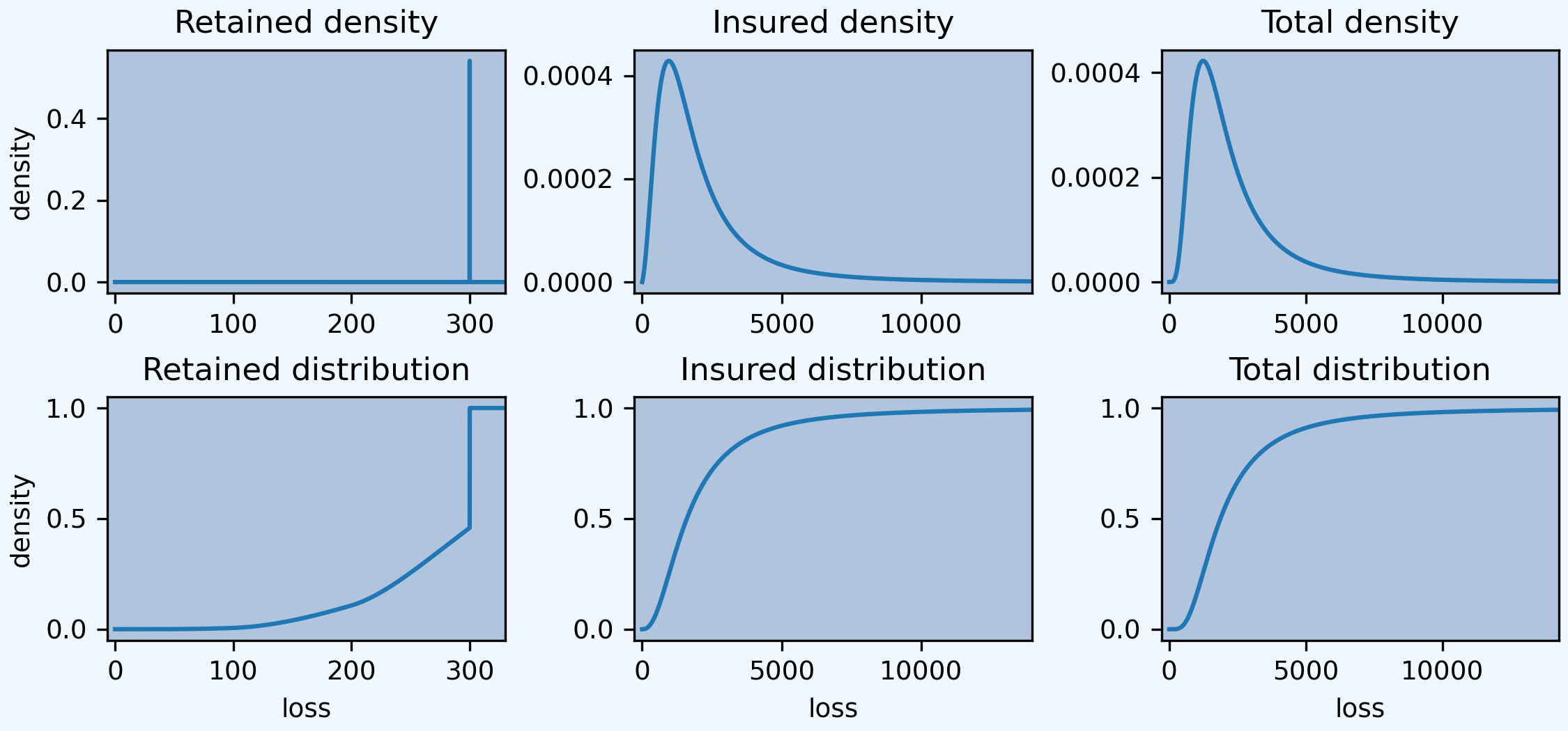
Compare the distributions by plotting the densities for (i) that retained, (ii) that accepted by the insurer, and (iii) the total overall amount.
Solution. Begin by figuring the gamma and Pareto parameters. For a gamma, the mean equals shape times scale, so shape equals 2 for building and motor. For a Pareto, the mean equals scale / (shape - 1), so shape equals 2 (no variance) for D&O and 3 for cyber (no third moment). We model the results using three Portfolio objects, one for the retention, one for the insured amount, and one total. In each case the distribution gives total losses; the frequency component is trivial.
Since the insured and total aggregates have no variance it is hard to estimate an appropriate bucket size. The default method uses the standard deviation as a scale factor. We must use judgement (or trial and error), and select log2=18 and bs=1 to ensure there is enough “space”. Checking the describe dataframe shows these values match the means well by unit and in total. The insured severity must be made unconditional.
In [110]: from aggregate import build

In [111]: retained = build('''port retained
   .....:     agg building 1 claim 100 xs 0 sev 100 * gamma 2 fixed
   .....:     agg motor    1 claim 200 xs 0 sev 200 * gamma 2 fixed
   .....: ''')
   .....:

In [112]: qd(retained)

                E[X] Est E[X]   Err E[X]   CV(X) Est CV(X) Skew(X) Est Skew(X)
unit     X
building Freq      1                           0
         Sev  89.636   89.636 1.0437e-10 0.23985   0.23985 -2.1029     -2.1029
         Agg  89.636   89.636 1.0437e-10 0.23985   0.23985 -2.1029     -2.1029
motor    Freq      1                           0
         Sev  179.27   179.27 2.6093e-11 0.23985   0.23985 -2.1029     -2.1029
         Agg  179.27   179.27 2.6093e-11 0.23985   0.23985 -2.1029     -2.1029
total    Freq      2                           0
         Sev  134.45   134.45 5.2187e-11 0.41837           -0.0046
         Agg  268.91   268.91 5.2187e-11 0.17878   0.17878 -1.6928     -1.6928
log2 = 16, bandwidth = 1/128, validation: not unreasonable.

In [113]: insured = build('''port insured
   .....:     agg building 1 claim inf xs 100 sev 100 * gamma 2 ! fixed
   .....:     agg motor    1 claim inf xs 200 sev 200 * gamma 2 ! fixed
   .....:     agg d.and.o  1 claim            sev 1000 * pareto 2 - 1000 fixed
   .....:     agg cyber    1 claim            sev 2000 * pareto 3 - 2000 fixed
   .....: ''', log2=18, bs=1)
   .....:

In [114]: qd(insured)

                E[X] Est E[X]    Err E[X]  CV(X) Est CV(X) Skew(X) Est Skew(X)
unit     X
building Freq      1                           0
         Sev  110.36   110.36 -1.3889e-06 1.1901    1.1901   1.757       1.757
         Agg  110.36   110.36 -1.3889e-06 1.1901    1.1901   1.757       1.757
motor    Freq      1                           0
         Sev  220.73   220.73 -3.4722e-07 1.1901    1.1901   1.757       1.757
         Agg  220.73   220.73 -3.4722e-07 1.1901    1.1901   1.757       1.757
d.and.o  Freq      1                           0
         Sev    1000   992.43  -0.0075717    inf    2.6992              24.633
         Agg    1000   992.43  -0.0075717    inf    2.6992              24.633
cyber    Freq      1                           0
         Sev    1000   999.83 -0.00017075 1.7321    1.7062     inf      12.894
         Agg    1000   999.83 -0.00017075 1.7321    1.7062     inf      12.894
total    Freq      4                           0
         Sev  582.77   580.84  -0.0033215    inf
         Agg  2331.1   2323.3  -0.0033392    inf    1.3721              16.508
log2 = 18, bandwidth = 1, validation: fails sev mean, agg mean.

In [115]: total = build('''port total
   .....:     agg building 1 claim sev 100 * gamma 2 fixed
   .....:     agg motor    1 claim sev 200 * gamma 2 fixed
   .....:     agg d.and.o  1 claim sev 1000 * pareto 2 - 1000 fixed
   .....:     agg cyber    1 claim sev 2000 * pareto 3 - 2000 fixed
   .....: ''', log2=18, bs=1)
   .....:

In [116]: qd(total)

               E[X] Est E[X]    Err E[X]   CV(X) Est CV(X) Skew(X) Est Skew(X)
unit     X
building Freq     1                            0
         Sev    200      200 -1.2153e-11 0.70711   0.70711  1.4142      1.4142
         Agg    200      200 -1.2153e-11 0.70711   0.70711  1.4142      1.4142
motor    Freq     1                            0
         Sev    400      400 -7.5939e-13 0.70711   0.70711  1.4142      1.4142
         Agg    400      400 -7.5939e-13 0.70711   0.70711  1.4142      1.4142
d.and.o  Freq     1                            0
         Sev   1000   992.43  -0.0075717     inf    2.6992              24.633
         Agg   1000   992.43  -0.0075717     inf    2.6992              24.633
cyber    Freq     1                            0
         Sev   1000   999.83 -0.00017075  1.7321    1.7062     inf      12.894
         Agg   1000   999.83 -0.00017075  1.7321    1.7062     inf      12.894
total    Freq     4                            0
         Sev    650   648.06  -0.0029779     inf
         Agg   2600   2592.2  -0.0029969     inf    1.2304              16.463
log2 = 18, bandwidth = 1, validation: fails sev mean, agg mean.
The spacing in the agg programs is for clarity. We could also program using dfreq as agg motor dfreq [1] 100 xs 0 sev.... Next, assemble the requested data elements.
In [117]: pfs = [retained, insured, total]

In [118]: answers = pd.DataFrame(columns=['retained', 'insured', 'total'])

In [119]: answers.index.name = 'statistic'

In [120]: answers.loc['expected claim amount'] = [x.agg_m for x in pfs]

In [121]: for p in [.8, .9, .95, .99]:
   .....:     answers.loc[f'claim p_{p:.2f}'] = [x.q(p) for x in pfs]
   .....:

In [122]: qd(answers)

                       retained  insured  total
statistic
expected claim amount    268.91   2331.1   2600
claim p_0.80                300     3090   3364
claim p_0.90                300     4483   4756
claim p_0.95                300     6244   6516
claim p_0.99                300    12706  12977
Finally, plot the densities. Compared to the text plot, the FFT reveals a discontinuous distribution for retained loss, with a large mass at 300. This is clearer on the lower plots, which show the distribution functions.
In [123]: fig, axs = plt.subplots(2, 3, figsize=(7.5, 3.5), constrained_layout=True, squeeze=True)

In [124]: xl = {}

In [125]: for ax, pf in zip(axs.flat, pfs):
   .....:     pf.density_df.p_total.plot(ax=ax)
   .....:     q = pf.q(0.99) * 1.1
   .....:     xl[hash(pf)] = [-q / 50, q]
   .....:     ax.set(xlim=xl[hash(pf)], title=pf.name.title() + ' density')
   .....:     if pf is retained:
   .....:         ax.set(ylabel='density')
   .....:

In [126]: for ax, pf in zip(axs.flat[3:], pfs):
   .....:     pf.density_df.F.plot(ax=ax)
   .....:     ax.set(xlim=xl[hash(pf)], title=pf.name.title() + ' distribution', xlabel='loss')
   .....:     if pf is retained:
   .....:         ax.set(ylabel='density')
   .....: