2.13.6. Bahnemann Monograph
Examples from the CAS published monograph Bahnemann [2015], Distributions for actuaries, which is a text for CAS Part 8. It is available for free on the [CAS Website](https://www.casact.org/monograph/cas-monograph-no-2).
2.13.6.1. Contents
Chapter 4: Aggregate Claims
2.13.6.2. Simple Discrete Aggregate, Example 4.1
Assume that n = 0, 1, 2 are the only possible numbers of claims and they occur with probabilities 0.6, 0.3 and 0.1, and that there exist just three potential claim sizes: 1, 2, and 3 with probabilities 0.4, 0.5 and 0.1. (Note: the text uses claim sizes 100, 200 and 300.) Compute the distribution of possible outcomes and its mean and variance.
Imports and convenience functions.
In [1]: from aggregate import build, qd, mv

In [2]: import matplotlib.pyplot as plt
Build the aggregate and display key statistics.
In [3]: a = build('agg Bahn.4.1 dfreq[0 1 2][.6 .3 .1] '
   ...:           'dsev[1 2 3][.4 .5 .1]')
   ...:

In [4]: qd(a)

      E[X] Est E[X]    Err E[X]   CV(X) Est CV(X)  Skew(X) Est Skew(X)
X
Freq   0.5                       1.3416            0.99381
Sev    1.7      1.7 -1.1102e-16 0.37665   0.37665  0.36568     0.36568
Agg   0.85     0.85 -2.2204e-16  1.4435    1.4435   1.3333      1.3333
log2 = 4, bandwidth = 1, validation: not unreasonable.

In [5]: mv(a)
mean     = 0.85
variance = 1.5055
std dev  = 1.22699
Display all possible outcomes. Compare with the table on p. 107.
In [6]: qd(a.density_df.query('p_total > 0') [['p_total', 'F']])

      p_total     F
loss
0.0       0.6   0.6
1.0      0.12  0.72
2.0     0.166 0.886
3.0      0.07 0.956
4.0     0.033 0.989
5.0      0.01 0.999
6.0     0.001     1
2.13.6.3. Poisson-Gamma (Tweedie) Aggregate, Example 4.2
The text considers a Tweedie with expected claim count \(\lambda=2.5\) and gammma shape 3 and scale 400. It computes the mean, variance and skewness, and uses the series expansion for the distribution to compute the CDF at various points (Table 4.1). These results can be replicated as follows.
In [7]: a = build('agg Bahn.4.2 2.5 claims '
   ...:           'sev 400 * gamma 3 poisson')
   ...:

In [8]: qd(a)

      E[X] Est E[X]    Err E[X]   CV(X) Est CV(X)  Skew(X) Est Skew(X)
X
Freq   2.5                      0.63246            0.63246
Sev   1200     1200  1.5543e-15 0.57735   0.57735   1.1547      1.1547
Agg   3000     3000 -2.7578e-13  0.7303    0.7303  0.91287     0.91287
log2 = 16, bandwidth = 1/2, validation: not unreasonable.

In [9]: mv(a)
mean     = 3000
variance = 4800000
std dev  = 2190.89
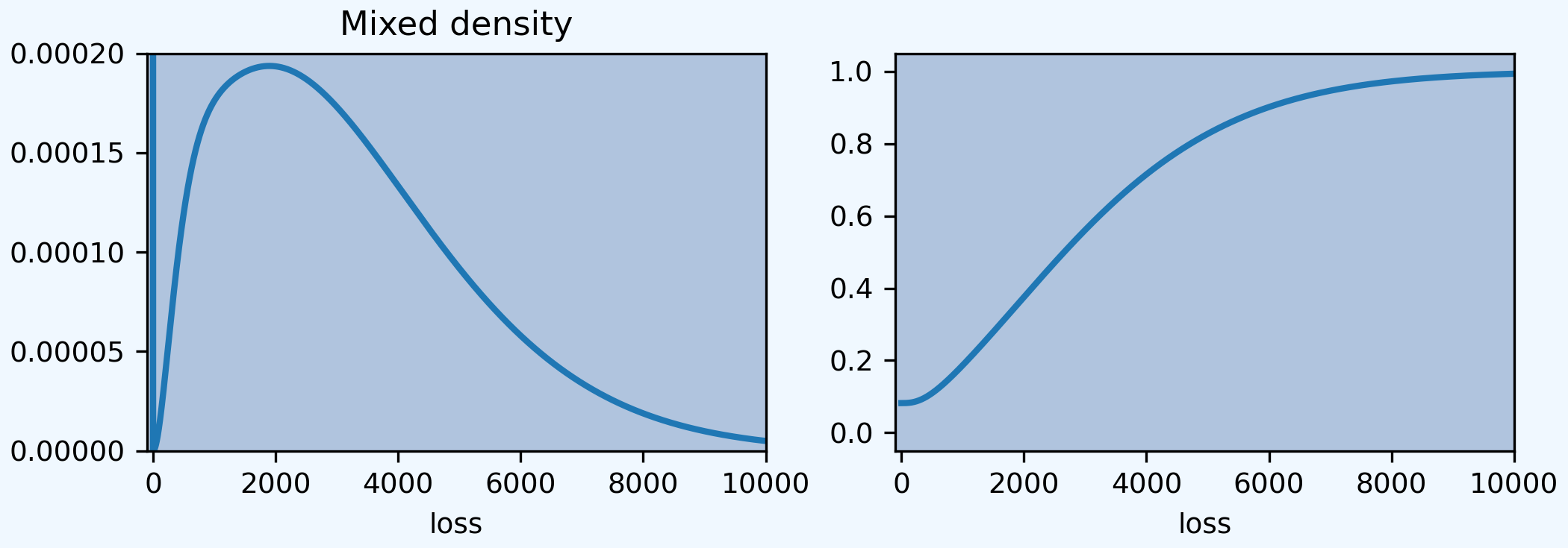
Extract various points of the pmf, cdf, and sf. The adjustment to the index is cosmetic. aggregate returns the entire distribution. The left plot shows the mixed density, with a mass at zero; right shows the cdf.
In [10]: bit = a.density_df.loc[
   ....:     sorted(np.hstack((500, np.arange(0, 10000.5, 1000)))),
   ....:     ['p', 'F', 'S']]
   ....:

In [11]: qd(bit, accuracy=4)

                 p        F        S
loss
0.0       0.082085 0.082085  0.91792
500.0   5.9764e-05  0.10958  0.89042
1000.0  8.8058e-05  0.18677  0.81323
2000.0  9.6726e-05  0.37558  0.62442
3000.0  8.6514e-05  0.56132  0.43868
4000.0  6.6611e-05  0.71519  0.28481
5000.0  4.5895e-05  0.82731  0.17269
6000.0  2.8971e-05  0.90135 0.098646
7000.0  1.7022e-05  0.94653 0.053468
8000.0  9.4148e-06  0.97234 0.027662
9000.0  4.9432e-06  0.98627 0.013727
10000.0 2.4799e-06  0.99344 0.006561

In [12]: fig, axs = plt.subplots(1, 2, figsize=(3.5*2, 2.45), constrained_layout=True, squeeze=True)

In [13]: ax0, ax1 = axs.flat

In [14]: (a.density_df.p / a.bs).plot(ylim=[0, 0.0002], xlim=[-100, 10000], lw=2, ax=ax0)
Out[14]: <Axes: xlabel='loss'>

In [15]: ax0.set(title='Density')
Out[15]: [Text(0.5, 1.0, 'Density')]

In [16]: a.density_df.F.plot(ylim=[-0.05, 1.05], xlim=[-100, 10000], lw=2, ax=ax1)
Out[16]: <Axes: xlabel='loss'>

In [17]: ax0.set(title='Mixed density');

In [18]: ax1.set(title='Distribution function');
2.13.6.4. Approximations to the Tweedie, Example 4.3
aggregate largely circumvents the need for approximations, but it does support their creation. The following reproduces Table 4.3.
In [19]: fz = a.approximate('all')

In [20]: bit['Normal'] = fz['norm'].cdf(bit.index)

In [21]: bit['Norm err'] = bit.Normal / bit.F - 1

In [22]: bit['sGamma'] = fz['sgamma'].cdf(bit.index)

In [23]: bit['sGamma err'] = bit.sGamma / bit.F - 1

In [24]: qd(bit, accuracy=4)

                 p        F        S   Normal   Norm err   sGamma  sGamma err
loss
0.0       0.082085 0.082085  0.91792 0.085452   0.041016 0.045932    -0.44044
500.0   5.9764e-05  0.10958  0.89042  0.12692    0.15821  0.10104   -0.077947
1000.0  8.8058e-05  0.18677  0.81323  0.18066  -0.032733  0.17751   -0.049594
2000.0  9.6726e-05  0.37558  0.62442  0.32404   -0.13723  0.36803   -0.020087
3000.0  8.6514e-05  0.56132  0.43868      0.5   -0.10924  0.56073  -0.0010453
4000.0  6.6611e-05  0.71519  0.28481  0.67596  -0.054848  0.71854   0.0046875
5000.0  4.5895e-05  0.82731  0.17269  0.81934 -0.0096235  0.83105   0.0045249
6000.0  2.8971e-05  0.90135 0.098646  0.91455   0.014639  0.90379   0.0027037
7000.0  1.7022e-05  0.94653 0.053468  0.96606   0.020626  0.94752   0.0010466
8000.0  9.4148e-06  0.97234 0.027662  0.98876    0.01689  0.97238  4.3133e-05
9000.0  4.9432e-06  0.98627 0.013727  0.99692    0.01079  0.98589 -0.00038586
10000.0 2.4799e-06  0.99344 0.006561   0.9993  0.0059007  0.99298 -0.00046669
Here is Table 4.4. The FFT overstates \(F(0)\) because of discretization error.
In [25]: a2 = build('agg Bahn.4.2b 10 claims '
   ....:            'sev 6000 * gamma 0.05 poisson')
   ....:

In [26]: qd(a2)

      E[X] Est E[X]    Err E[X]   CV(X) Est CV(X)  Skew(X) Est Skew(X)
X
Freq    10                      0.31623            0.31623
Sev    300   299.94 -0.00018672  4.4721     4.473   8.9443      8.9441
Agg   3000   2999.4 -0.00018672  1.4491    1.4494   2.8293      2.8293
log2 = 16, bandwidth = 5, validation: fails sev mean, agg mean.

In [27]: fz = a2.approximate('all')

In [28]: bit = a2.density_df.loc[
   ....:     sorted(np.hstack((500, np.arange(0, 20000, 2000)))),
   ....:     ['p', 'F', 'S']]
   ....:

In [29]: bit['Normal'] = fz['norm'].cdf(bit.index)

In [30]: bit['Norm err'] = bit.Normal / bit.F - 1

In [31]: bit['sGamma'] = fz['sgamma'].cdf(bit.index)

In [32]: bit['sGamma err'] = bit.sGamma / bit.F - 1

In [33]: qd(bit, accuracy=4)

                 p        F        S  Normal  Norm err  sGamma  sGamma err
loss
0.0       0.047861 0.047861  0.95214 0.24512    4.1215 0.12322      1.5746
500.0    0.0014101  0.33964  0.66036 0.28267  -0.16774 0.33446   -0.015242
2000.0  0.00055391  0.59253  0.40747 0.40909  -0.30959  0.5887  -0.0064723
4000.0  0.00028651  0.75148  0.24852 0.59101  -0.21353 0.75043  -0.0013915
6000.0  0.00017056  0.84025  0.15975 0.75496   -0.1015 0.84022 -3.1891e-05
8000.0  0.00010741  0.89466  0.10534 0.87498 -0.022001 0.89493  0.00030275
10000.0 6.9725e-05  0.92946 0.070541 0.94633  0.018153 0.92976   0.0003232
12000.0 4.6131e-05  0.95227 0.047735 0.98079  0.029954 0.95251  0.00025575
14000.0 3.0919e-05  0.96745 0.032549  0.9943  0.027755 0.96762  0.00017682
16000.0 2.0919e-05  0.97768 0.022323 0.99861  0.021408 0.97779  0.00011036
18000.0 1.4255e-05  0.98462  0.01538 0.99972  0.015336 0.98468  6.1254e-05
2.13.6.5. Poisson-Discrete Distribution, Example 4.4
The claim-count random variable is Poisson distributed with mean 1.75. Severity has a discrete distribution with outcomes 1, 2, 3, 4, 5 occurring with probabilities 0.2, 0.4, 0.2, 0.15, 0.05 respectively. Compute the aggregate distribution.
Here is Table 4.5.
In [34]: a = build('agg Bahn.4.4 1.75 claims '
   ....:           'dsev [1 2 3 4 5] [.2 .4 .2 .15 .05] '
   ....:           'poisson')
   ....:

In [35]: qd(a)

       E[X] Est E[X]    Err E[X]   CV(X) Est CV(X)  Skew(X) Est Skew(X)
X
Freq   1.75                      0.75593            0.75593
Sev    2.45     2.45 -2.2204e-16 0.45588   0.45588  0.55603     0.55603
Agg  4.2875   4.2875  2.2204e-16 0.83078   0.83078  0.95453     0.95453
log2 = 7, bandwidth = 1, validation: not unreasonable.

In [36]: qd(a.density_df.query('p > .001')[['p', 'F', 'S']], accuracy=4)

             p       F         S
loss
0.0    0.17377 0.17377   0.82623
1.0   0.060821 0.23459   0.76541
2.0    0.13229 0.36688   0.63312
3.0    0.10464 0.47152   0.52848
4.0    0.11704 0.58855   0.41145
5.0   0.093249  0.6818    0.3182
6.0   0.078644 0.76045   0.23955
7.0   0.064101 0.82455   0.17545
8.0   0.049889 0.87444   0.12556
9.0   0.037655 0.91209  0.087908
10.0   0.02737 0.93946  0.060537
11.0  0.019672 0.95913  0.040865
12.0  0.013764  0.9729  0.027101
13.0 0.0094201 0.98232  0.017681
14.0 0.0063168 0.98864  0.011364
15.0 0.0041654  0.9928 0.0071986
16.0 0.0027032  0.9955 0.0044954
17.0 0.0017249 0.99723 0.0027705
18.0 0.0010842 0.99831 0.0016863
2.13.6.6. Poisson-Gamma Distribution, Example 4.5
Aggregate losses have Poisson frequency with mean 2.5 and gamma severity with shape 3 and scale 400. Hence the aggregate mean equals 1,200 and variance equals 480,000.
Now approximate the distribution function using FFT with a fine bucket size and the midpoint method for assigning claim-size probabilities and then bs=20 and bs=100.
Here is Table 4.6, comparing the distributions. The update method re-runs the FFT computation with different options, here altering bs.
In [37]: import numpy as np

In [38]: import pandas as pd

In [39]: a = build('agg Bahn.4.5 2.5 claims '
   ....:           'sev 400 * gamma 3 poisson')
   ....:

In [40]: qd(a)

      E[X] Est E[X]    Err E[X]   CV(X) Est CV(X)  Skew(X) Est Skew(X)
X
Freq   2.5                      0.63246            0.63246
Sev   1200     1200  1.5543e-15 0.57735   0.57735   1.1547      1.1547
Agg   3000     3000 -2.7578e-13  0.7303    0.7303  0.91287     0.91287
log2 = 16, bandwidth = 1/2, validation: not unreasonable.

In [41]: xs = sorted(np.hstack((500, np.arange(0, 10001, 1000))))

In [42]: bit = a.density_df.loc[xs, ['F']]

In [43]: a.update(bs=100)

In [44]: bit100 = a.density_df.loc[xs,  ['F']]

In [45]: a.update(bs=20)

In [46]: bit20 = a.density_df.loc[xs,  ['F']]

In [47]: bit = pd.concat((bit, bit100, bit20), axis=1, keys=['h0.25', 'h100', 'h20'])

In [48]: bit[('h100', 'Rel Error')] = bit[('h100', 'F')] / bit[('h0.25', 'F')] - 1

In [49]: bit[('h20', 'Rel Error')] = bit[('h20', 'F')] / bit[('h0.25', 'F')] - 1

In [50]: bit = bit.sort_index(axis=1)

In [51]: qd(bit, accuracy=4)

           h0.25     h100                 h20
               F        F  Rel Error        F  Rel Error
loss
0.0     0.082085 0.082146 0.00074147 0.082086 6.3895e-06
500.0    0.10958  0.11579   0.056708  0.11076   0.010735
1000.0   0.18677  0.19565   0.047526  0.18849  0.0092186
2000.0   0.37558  0.38525   0.025749  0.37747  0.0050273
3000.0   0.56132  0.56991   0.015294  0.56301   0.003004
4000.0   0.71519  0.72175  0.0091789  0.71648  0.0018127
5000.0   0.82731   0.8318  0.0054318   0.8282  0.0010783
6000.0   0.90135  0.90417  0.0031276  0.90192 0.00062395
7000.0   0.94653  0.94818  0.0017394  0.94686 0.00034868
8000.0   0.97234  0.97324 0.00093101  0.97252  0.0001875
9000.0   0.98627  0.98675 0.00047913  0.98637 9.6942e-05
10000.0  0.99344  0.99367 0.00023728  0.99349 4.8226e-05
2.13.6.7. Poisson-Lognormal Distribution With Limit, Example 4.15
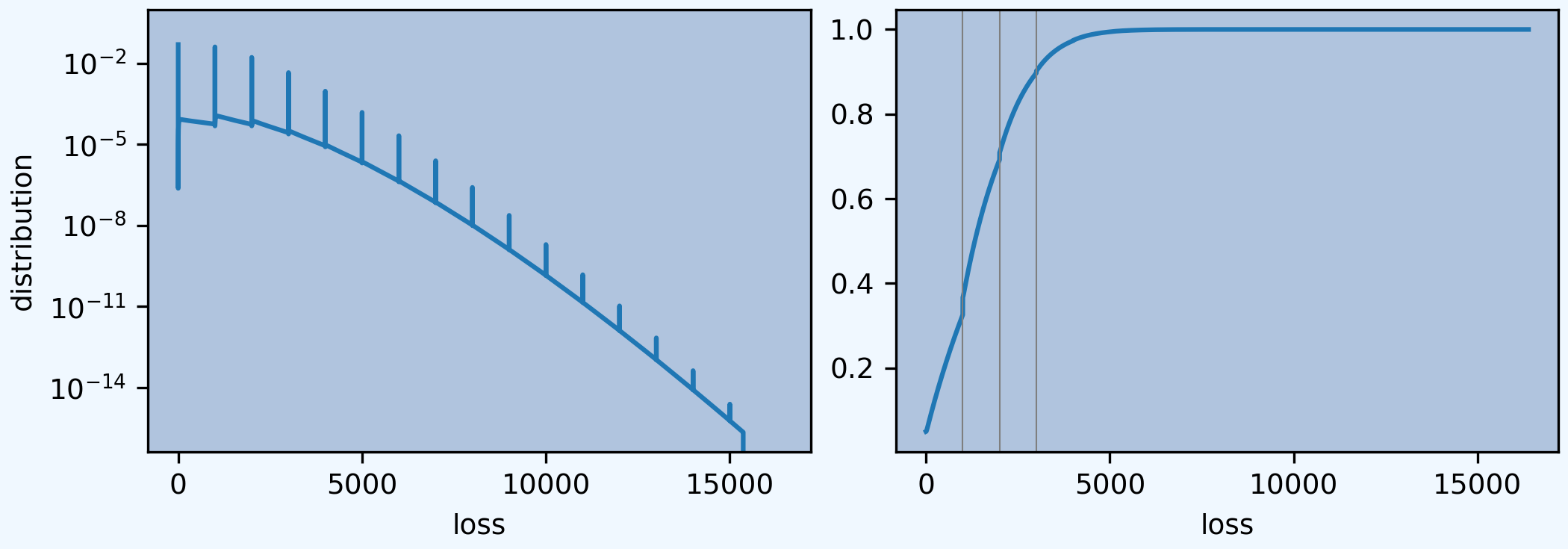
Consider an aggregate distribution with mean 3 Poisson frequency and lognormal claim size with parameters \((\mu, \sigma) = (6, 1.5)\). Moreover, claim size is limited by a policy limit of 1,000. Graph the aggregate distribution.
The log density (left) shows the probability masses at outcomes consisting of only limit losses. The distribution (right) shows the corresponding jumps. Compare with Figure 4.4.
In [52]: a = build('agg Bahn.4.15 '
   ....:           '3 claims '
   ....:           '1000 xs 0 '
   ....:           'sev exp(6) * lognorm 1.5 '
   ....:           'poisson')
   ....:

In [53]: qd(a)

       E[X] Est E[X]   Err E[X]   CV(X) Est CV(X)  Skew(X) Est Skew(X)
X
Freq      3                     0.57735            0.57735
Sev  502.97   502.97 1.1478e-09 0.74753   0.74753  0.23542     0.23542
Agg  1508.9   1508.9 1.1478e-09 0.72083   0.72083  0.82314     0.82314
log2 = 16, bandwidth = 1/4, validation: not unreasonable.

In [54]: fig, axs = plt.subplots(1, 2, figsize=(2*3.5, 2.45), constrained_layout=True)

In [55]: ax0, ax1 = axs.flat

In [56]: a.density_df.p.plot(ax=ax0, logy=True, label='FFT');

In [57]: a.density_df.F.plot(ax=ax1, label='FFT');

In [58]: ax0.set(ylabel='log density');

In [59]: ax0.set(ylabel='distribution', ylim=[0,1]);

In [60]: ax1.axvline(1000, c='C7', lw=.5);

In [61]: ax1.axvline(2000, c='C7', lw=.5);

In [62]: ax1.axvline(3000, c='C7', lw=.5);
2.13.6.8. Poisson-Gamma Distribution and Approximations, Problems 4.7 and 13
An aggregate distribution has mean 8 Poisson frequency and gamma severity with shape 0.2 and scale 3750. Compute the distribution and compare with normal and shifted-gamma approximations.
In [63]: a = build('agg Bahn.4.7 '
   ....:       '8 claims '
   ....:       'sev 3750 * gamma 0.2 '
   ....:       'poisson')
   ....:

In [64]: qd(a)

      E[X] Est E[X]    Err E[X]   CV(X) Est CV(X)  Skew(X) Est Skew(X)
X
Freq     8                      0.35355            0.35355
Sev    750   749.98 -2.9119e-05  2.2361    2.2361   4.4721      4.4721
Agg   6000   5999.8 -2.9119e-05 0.86603   0.86605   1.5877      1.5877
log2 = 16, bandwidth = 2, validation: not unreasonable.

In [65]: xs = np.arange(0, 30000,3000)

In [66]: qd(a.density_df.loc[xs, ['p', 'F','S']], accuracy=4)

                 p         F         S
loss
0.0      0.0018002 0.0018002    0.9982
3000.0  0.00020926   0.34209   0.65791
6000.0  0.00014322   0.60704   0.39296
9000.0  8.7227e-05    0.7775    0.2225
12000.0 5.0019e-05   0.87823   0.12177
15000.0 2.7618e-05   0.93494  0.065065
18000.0 1.4853e-05   0.96586  0.034143
21000.0 7.8339e-06   0.98233  0.017666
24000.0 4.0696e-06   0.99096 0.0090364
27000.0 2.0885e-06   0.99542 0.0045787
aggregate readily computes approximations and returns frozen scipy.stats objects.
In [67]: fz = a.approximate('all')

In [68]: comp = pd.DataFrame({k: v.cdf(xs) for k, v in fz.items()}, index=xs)

In [69]: comp['agg'] = a.density_df.loc[xs, 'F',]

In [70]: comp.loc[:, [f'{k} err' for k in fz.keys()]] = comp.loc[:, fz.keys()].values / comp.loc[:, ['agg']].values - 1

In [71]: comp = comp.sort_index(axis=1)

In [72]: qd(comp, accuracy=4)

            agg   gamma   gamma err  lognorm  lognorm err    norm   norm err   sgamma  sgamma err  \
0     0.0018002       0          -1        0           -1 0.12411     67.945 0.026306      13.613
3000    0.34209 0.33977  -0.0067746  0.29031     -0.15135 0.28186   -0.17605  0.33624   -0.017089
6000    0.60704 0.61485    0.012868  0.64583     0.063894 0.50001   -0.17631  0.60542  -0.0026701
9000     0.7775 0.78363   0.0078835  0.82019     0.054907 0.71816   -0.07632  0.77824  0.00095764
12000   0.87823 0.88084   0.0029796  0.90331      0.02856  0.8759 -0.0026494  0.87926   0.0011727
15000   0.93494  0.9352  0.00028096  0.94508     0.010852 0.95837   0.025066  0.93559   0.0007034
18000   0.96586 0.96506 -0.00082253  0.96731    0.0015039 0.98954   0.024521  0.96614  0.00028959
21000   0.98233 0.98128  -0.0010704  0.97975   -0.0026265 0.99805   0.016002  0.98239  5.1729e-05
24000   0.99096 0.99002 -0.00095081  0.98703   -0.0039667 0.99973  0.0088504  0.99091 -5.1265e-05
27000   0.99542  0.9947 -0.00072386  0.99145   -0.0039875 0.99997  0.0045731  0.99534  -7.866e-05

       slognorm  slognorm err
0      0.058626        31.567
3000    0.31389     -0.082441
6000    0.59173     -0.025232
9000    0.77906      0.002005
12000   0.88465     0.0073188
15000   0.94022     0.0056501
18000   0.96881     0.0030552
21000    0.9835      0.001191
24000   0.99113     0.0001684
27000   0.99515   -0.00027715
2.13.6.9. Poisson-Lognormal Layer Statistics, Example 5.13
Consider an aggregate distribution with mean 15 Poisson frequency and lognormal claim size with parameters \((\mu, \sigma) = (5.9809, 1.8)\). What are the distribution characteristics for random variable S for claims in the layer 5,000 excess of 3,000?
The exact and FFT-estimated mean, cv, and skewness are reported in the describe dataframe, for frequency and severity. The values reported agree with the text, up to rounding.
In [73]: a = build('agg Bahn.5.13 '
   ....:       '15 claims 5000 xs 3000 '
   ....:       'sev exp(5.9809) * lognorm 1.8 ! '
   ....:       'poisson')
   ....:

In [74]: qd(a)

       E[X] Est E[X]    Err E[X]   CV(X) Est CV(X)  Skew(X) Est Skew(X)
X
Freq     15                       0.2582             0.2582
Sev  385.68   385.68 -3.4957e-09  3.1319    3.1319   3.1942      3.1942
Agg  5785.3   5785.3 -3.4982e-09 0.84887   0.84887  0.93405     0.93405
log2 = 16, bandwidth = 1, validation: not unreasonable.

In [75]: mv(a)
mean     = 5785.25
variance = 2.411727e+07
std dev  = 4910.93
The exact severity can be accessed directly, as a.sevs[0].fz, allowing us to compute the expected layer claim count. The aggregate can then be written in conditional form, producing the same statistics. The distribution function shows probability masses at multiples of the limit.
In [76]: xs = 15 * a.sevs[0].fz.sf(3000)

In [77]: print(f'excess claim count = {xs:.5f}')
excess claim count = 1.95359

In [78]: a = build('agg Bahn.5.13b '
   ....:           f'{xs} claims 5000 xs 3000 '
   ....:           'sev exp(5.9809) * lognorm 1.8 '
   ....:           'poisson')
   ....:

In [79]: qd(a)

       E[X] Est E[X]    Err E[X]   CV(X) Est CV(X)  Skew(X) Est Skew(X)
X
Freq 1.9536                      0.71546            0.71546
Sev  2961.3   2961.3 -3.4956e-09 0.63853   0.63853 -0.16374    -0.16374
Agg  5785.3   5785.3 -3.4982e-09 0.84887   0.84887  0.93405     0.93405
log2 = 16, bandwidth = 1, validation: not unreasonable.

In [80]: fig, ax = plt.subplots(1,1,figsize=(3.5, 2.45))

In [81]: a.density_df.F.plot(ax=ax, label='FFT');

In [82]: fz = a.approximate('gamma')

In [83]: ax.plot(a.density_df.loss, fz.cdf(a.density_df.loss), c='C1', label='gamma approx.');

In [84]: ax.axvline(5000,  c='C7', lw=.5);

In [85]: ax.axvline(10000, c='C7', lw=.5);

In [86]: ax.axvline(15000, c='C7', lw=.5);

In [87]: ax.set(ylabel='cdf');

In [88]: ax.legend(loc='lower right');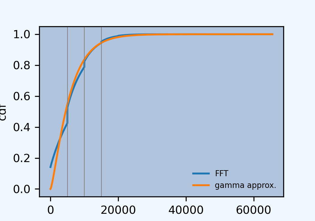
2.13.6.10. Lognormal Increased Limits Factors (ILFs), Example 6.3
Indemnity losses for a portfolio of insurance policies have a lognormal claim-size distribution with parameters \((\mu, \sigma) = (7, 2.4)\). The policy per-claim limit applies only to the indemnity portion of a claim, and the average per-claim loss adjustment expense is 2,200. Claim frequency for these policies is 0.0005 per exposure unit, and variable expenses equal 35% of premium.
A lognormal with \(\sigma = 2.4\) has cv \(\sqrt{\exp(2.4^2)-1}=17.78\) and is extremely thick-tailed, despite having moments of all orders. It is challenging to approximate numerically. Luckily, we only need to compute up to 5M. The aggregate parameters deliberately select a range that is too narrow for the entire distribution, but adequate for our purposes. Use log2=17 and select bs greater than 5e6 // 2**17 = 38. We use bs=50.
It is important to set normalize=False to avoid rescaling bucket probabilities to sum to one. These parameters are not a good model for the entire distribution; the mean error is too high.
The density_df dataframe includes limited expected values. Here is a sample.
In [89]: a = build('agg Bahn.6.3 '
   ....:           '1 claim '
   ....:           'sev exp(7) * lognorm 2.4 '
   ....:           'fixed',
   ....:           bs=50, log2=17,
   ....:           normalize=False,
   ....:          )
   ....:

In [90]: qd(a)

      E[X] Est E[X]  Err E[X]  CV(X) Est CV(X) Skew(X) Est Skew(X)
X
Freq     1                         0
Sev  19536    18328 -0.061835 17.786    7.7935    5680      27.885
Agg  19536    18328 -0.061835 17.786    7.7935    5680      27.885
log2 = 17, bandwidth = 50, validation: fails sev mean, agg mean.

In [91]: xs = [1e5,  5e5, 7.5e5, 1e6, 2e6, 3e6, 4e6, 5e6]

In [92]: qd(a.density_df.loc[xs, ['F', 'S', 'lev']], accuracy=4)

                F          S    lev
loss
100000.0  0.96998   0.030021 8895.8
500000.0  0.99463  0.0053706  13625
750000.0  0.99674  0.0032647  14668
1000000.0 0.99774   0.002257  15345
2000000.0 0.99912 0.00087817  16738
3000000.0 0.99951 0.00048765  17390
4000000.0 0.99968 0.00031609  17782
5000000.0 0.99978 0.00022372  18048
The following reproduces Table 6.1. The ILF factors assume fixed (middle) and variable ALAE (right).
In [93]: alae = 2200

In [94]: bit = a.density_df.loc[xs, ['lev']]

In [95]: bit['Fixed ALAE'] = (bit.lev + alae) / (bit.lev.iloc[0] + alae)

In [96]: bit['Prop ALAE'] = bit.lev / bit.lev.iloc[0]

In [97]: qd(bit, accuracy=4)

             lev  Fixed ALAE  Prop ALAE
loss
100000.0  8895.8           1          1
500000.0   13625      1.4262     1.5317
750000.0   14668      1.5202     1.6488
1000000.0  15345      1.5812      1.725
2000000.0  16738      1.7067     1.8815
3000000.0  17390      1.7655     1.9549
4000000.0  17782      1.8009     1.9989
5000000.0  18048      1.8248     2.0288
2.13.6.12. Risk Loads, Example 6.5
Example 6.5, computes risk loads as a percentage of standard deviation. aggregate can compute multiple limits at once, and the report_df dataframe returns individual severity and aggregate distribution statistics. The risk loads can be deduced from these. The risk load can be computed as k' * ex2 or k * agg_cv (not shown).
The following code reproduces Table 6.3. First, define the controlling variables, and then set up the tower of limits within one object, using Vectorization: Limit Profiles and Mixed Severity.
In [104]: k_prime = 0.0277

In [105]: m = 400

In [106]: ϕ = 0.0005

In [107]: u = 0.2

In [108]: k = k_prime / np.sqrt(m * ϕ)

In [109]: limits = [1e5, 5e5, 1e6, 2e6, 3e6, 4e6, 5e6]

In [110]: bl = build('agg Bahn.6.5 '
   .....:            f'{m * ϕ} claims '
   .....:            f'{limits} xs 0 '
   .....:            'sev exp(7) * lognorm 2.4 '
   .....:            'poisson'
   .....:            , bs=50, log2=18)
   .....:

In [111]: qd(bl.report_df.iloc[:, :-4], accuracy=4)

view               0         1         2         3         4         5         6
statistic
name        Bahn.6.5  Bahn.6.5  Bahn.6.5  Bahn.6.5  Bahn.6.5  Bahn.6.5  Bahn.6.5
limit          1e+05     5e+05     1e+06     2e+06     3e+06     4e+06     5e+06
attachment         0         0         0         0         0         0         0
el            1779.2    2725.1      3069    3347.6      3478    3556.5    3609.6
freq_m           0.2       0.2       0.2       0.2       0.2       0.2       0.2
freq_cv       2.2361    2.2361    2.2361    2.2361    2.2361    2.2361    2.2361
freq_skew     2.2361    2.2361    2.2361    2.2361    2.2361    2.2361    2.2361
sev_m           8896     13626     15345     16738     17390     17782     18048
sev_cv        2.3401    3.7719      4.63    5.6565    6.3357     6.851    7.2685
sev_skew      3.3416    7.0585    9.9524    14.303    17.849    20.975    23.827
agg_m         1779.2    2725.1      3069    3347.6      3478    3556.5    3609.6
agg_cv        5.6903    8.7257    10.592    12.844    14.342    15.482    16.406
agg_skew      8.1747    15.898    22.157    31.683    39.494    46.396    52.704
Next, extract the required columns from report_df and manipulate to compute the ILFs.
In [112]: bit = bl.report_df.loc[['sev_m', 'sev_cv', 'agg_m', 'agg_cv']].iloc[:, :-4].T

In [113]: bit.index = limits

In [114]: bit.index.name = 'limit'

In [115]: bit['vx'] = (bit.sev_m * bit.sev_cv) ** 2

In [116]: bit['ex2'] = bit.vx + bit.sev_m**2

In [117]: bit['risk load'] = k_prime * bit.ex2 ** 0.5

In [118]: bit['lev'] = (1+u) * bit.sev_m

In [119]: bit['ILF w/o risk'] = bit['lev'] / bit.loc[100000, 'lev']

In [120]: bit['ILF with risk'] = (bit['lev'] + bit['risk load']) / (bit.loc[100000, 'lev'] + bit.loc[100000, 'risk load'])

In [121]: qd(bit, accuracy=4)

statistic sev_m sev_cv  agg_m agg_cv         vx        ex2 risk load   lev ILF w/o risk  \
limit
100000.0   8896 2.3401 1779.2 5.6903 4.3337e+08 5.1251e+08    627.09 10675            1
500000.0  13626 3.7719 2725.1 8.7257 2.6414e+09 2.8271e+09    1472.8 16351       1.5316
1000000.0 15345   4.63   3069 10.592 5.0478e+09 5.2833e+09    2013.4 18414       1.7249
2000000.0 16738 5.6565 3347.6 12.844  8.964e+09 9.2441e+09    2663.3 20085       1.8815
3000000.0 17390 6.3357   3478 14.342 1.2139e+10 1.2442e+10    3089.7 20868       1.9548
4000000.0 17782  6.851 3556.5 15.482 1.4842e+10 1.5158e+10    3410.4 21339       1.9989
5000000.0 18048 7.2685 3609.6 16.406 1.7208e+10 1.7534e+10    3667.9 21658       2.0288

statistic ILF with risk
limit
100000.0              1
500000.0          1.577
1000000.0        1.8074
2000000.0        2.0127
3000000.0        2.1197
4000000.0        2.1897
5000000.0        2.2407
2.13.6.14. Deductible Credits, Example 6.7
(Continues Example 6.3.) Consider a portfolio of policies for which the ground-up indemnity claim size has a lognormal distribution with parameters \((\mu, \sigma) = (7.0, 2.4)\) and allocated loss adjustment expense is 20% of the indemnity amount. The basic limit is 100,000. Calculate the credit factors, as well as the resulting frequency and severity, for six straight deductible options: 1,000; 2,000; 3,000; 4,000; 5,000; and 10,000. Base frequency equals 0.0005.
We can build all of the required distributions simultaneously using vectorization. Remember that the basic limit is ground up. The severity is unconditional, indicated by ! at the end of the severity clause. The limit is eroded by the deductible.
In [138]: deductibles = [0, 1e3, 2e3, 3e3, 4e3, 5e3, 10e3]

In [139]: limits = [100000 - i for i in deductibles]

In [140]: ϕ = 0.0005

In [141]: alae = 1.2

In [142]: bl = build('agg Bahn.6.7 '
   .....:            f'{ϕ} claims '
   .....:            f'{limits} xs {deductibles} '
   .....:            'sev exp(7) * lognorm 2.4 ! '
   .....:            'poisson'
   .....:            , bs=50, log2=18)
   .....:

In [143]: qd(bl.report_df.iloc[:, :-4], accuracy=4)

view               0         1         2         3         4         5         6
statistic
name        Bahn.6.7  Bahn.6.7  Bahn.6.7  Bahn.6.7  Bahn.6.7  Bahn.6.7  Bahn.6.7
limit          1e+05     99000     98000     97000     96000     95000     90000
attachment         0      1000      2000      3000      4000      5000     10000
el             4.448    4.1183    3.8926    3.7092    3.5517    3.4124    2.8758
freq_m        0.0005    0.0005    0.0005    0.0005    0.0005    0.0005    0.0005
freq_cv       44.721    44.721    44.721    44.721    44.721    44.721    44.721
freq_skew     44.721    44.721    44.721    44.721    44.721    44.721    44.721
sev_m           8896    8236.6    7785.2    7418.4    7103.4    6824.9    5751.7
sev_cv        2.3401    2.5106    2.6287    2.7269     2.813    2.8907    3.2067
sev_skew      3.3416    3.3681    3.4054    3.4444    3.4833    3.5215    3.6997
agg_m          4.448    4.1183    3.8926    3.7092    3.5517    3.4124    2.8758
agg_cv        113.81    120.85    125.78    129.89    133.51    136.79    150.22
agg_skew      163.49    165.89    168.03    170.02    171.89    173.66    181.54
Next, manipulate the report_df dataframe to compute the required quantities. The final exhibit replicates Table 6.5.
In [144]: bit = bl.report_df.iloc[:, :-4].loc[['attachment', 'freq_m', 'sev_m', 'agg_m']].T

In [145]: bit = bit.rename(columns={'attachment': 'deductible'}).set_index('deductible')

In [146]: bit['F(d)'] = np.array([bl.sevs[0].fz.cdf(i) for i in bit.index])

In [147]: bit['freq_m'] = bit.loc[0, 'freq_m'] * (1 - bit['F(d)'])

In [148]: bit['E[X;d]'] = (bit.sev_m[0] - bit.sev_m)

In [149]: bit['C(d)'] = bit['E[X;d]'] / bit.sev_m[0]

In [150]: bit['sev_m'] = bit['sev_m'] / (1 - bit['F(d)']) * alae

In [151]: bit = bit.iloc[:, [-2, 3, -1, 0, 1]]

In [152]: bit['pure prem'] = bit.freq_m * bit.sev_m

In [153]: qd(bit, accuracy=4)

statistic  E[X;d]    F(d)     C(d)     freq_m sev_m pure prem
deductible
0.0             0       0        0     0.0005 10675    5.3376
1000.0     659.42 0.48467 0.074125 0.00025766 19180     4.942
2000.0     1110.8 0.59885  0.12487 0.00020057 23289    4.6711
3000.0     1477.7 0.66251  0.16611 0.00016875 26377     4.451
4000.0     1792.7 0.70512  0.20151 0.00014744 28907     4.262
5000.0     2071.2 0.73636  0.23282 0.00013182 31064    4.0949
10000.0    3144.4 0.82147  0.35346 8.9266e-05 38660     3.451
2.13.6.15. Summary
Here is a summary of all the objects created in this section.
In [154]: from aggregate import pprint_ex

In [155]: for n, r in build.qlist('^Bahn').iterrows():
   .....:     pprint_ex(r.program, split=20)
   .....: