2.4.11. The tweedie Keyword
Prerequisites: Tweedie distribution from GLMs. Use of build.
See also: The Tweedie Distribution.
The aggregate language keyword tweedie makes it easy to build Tweedie distributions.
It uses reproductive
parameters \(\mu, p, \sigma^2\) (mean, power, and dispersion), since these are most natural for GLM modeling.
Example.
The keyword is used as follows to produce \(\mathsf{Tw}_{1.05}(2, 5)\), mean 2, \(p=1.05\), and dispersion 5.
In [1]: from aggregate import build, qd, mv

In [2]: a15 = build('agg DecL:15 tweedie 2 1.05 5')

In [3]: qd(a15)

        E[X] Est E[X]    Err E[X]   CV(X) Est CV(X)  Skew(X) Est Skew(X)
X
Freq 0.40671                        1.568              1.568
Sev   4.9175   4.9175 -2.3315e-15 0.22942   0.22942  0.45883     0.45883
Agg        2        2 -2.2204e-15  1.6088    1.6088   1.6892      1.6892
log2 = 16, bandwidth = 1/512, validation: not unreasonable.

In [4]: mv(a15)
mean     = 2
variance = 10.35265
std dev  = 3.21755

In [5]: print(f'Expected variance = disp x mean ** p = {2**1.05 * 5:.5f}')
Expected variance = disp x mean ** p = 10.35265
Inspecting the (non-trivial parts of the) specification shows the parser converts it into the additive form:
In [6]: {k: v for k,v in a15.spec.items()
   ...:     if v!=0 and v is not None and v!=''}
   ...:
Out[6]:
{'name': 'DecL:15',
 'exp_en': 0.4067100332315139,
 'exp_limit': inf,
 'sev_name': 'gamma',
 'sev_a': 18.999999999999982,
 'sev_scale': 0.2588162309603446,
 'sev_wt': 1,
 'sev_ub': inf,
 'sev_conditional': True,
 'freq_name': 'poisson',
 'freq_p0': nan,
 'note': 'Tw(p=1.05, μ=2.0, σ^2=5.0) --> CP(λ= 0.40671, ga(α=19, β=0.25881623), scale=0.25881623'}
The note shows the compound Poisson specification.
The helper function tweedie_convert translates between parameterizations. The scale (dispersion) parameter \(\sigma^2\) has offsetting effects: higher \(\sigma^2\) results in a lower claim count, a higher gamma mean, and a more skewed aggregate distribution with a bigger mass at zero.
Example.
The code below shows the three Tweedie representations, starting with the easiest to interpret.
In [7]: from aggregate import tweedie_convert

In [8]: import pandas as pd

In [9]: p = 1.005; μ = 1; σ2 = 0.1;                    \
   ...: m0 = tweedie_convert(p=p, μ=μ, σ2=σ2);         \
   ...: λ = μ**(2-p) / ((2-p) * σ2);                   \
   ...: α = (2 - p) / (p - 1);                         \
   ...: β = μ / (λ * α);                               \
   ...: tw_cv = σ2**.5 * μ**(p/2-1);                   \
   ...: sev_m = α *  β;                                \
   ...: sev_cv = α**-0.5;                              \
   ...: m1 = tweedie_convert(λ=λ, m=sev_m, cv=sev_cv); \
   ...: m2 = tweedie_convert(λ=λ, α=α, β=β);
   ...:

In [10]: assert np.allclose(m0, m1, m2)

In [11]: temp = pd.concat((m0, m1, m2), axis=1); \
   ....: temp.columns = ['mean p disp', 'lambda sev m cv', 'lambda shape scale'];
   ....:

In [12]: with pd.option_context('display.float_format', lambda x: f'{x:.12g}'):
   ....:     print(temp)
   ....:
             mean p disp   lambda sev m cv  lambda shape scale
μ                      1                 1                   1
p                  1.005             1.005               1.005
σ^2                  0.1               0.1                 0.1
λ          10.0502512563     10.0502512563       10.0502512563
α                    199               199                 199
β                 0.0005            0.0005              0.0005
tw_cv     0.316227766017    0.316227766017      0.316227766017
sev_m             0.0995            0.0995              0.0995
sev_cv   0.0708881205008   0.0708881205008     0.0708881205008
p0     4.31748997327e-05 4.31748997327e-05   4.31748997327e-05
Three different ways of specifying the same Tweedie distribution.
In [13]: program = f'''
   ....: agg DecL:16 {λ} claims sev gamma {sev_m:.8g} cv {sev_cv} poisson
   ....: agg DecL:17 {λ} claims sev {β:.4g} * gamma {α:.4g} poisson
   ....: agg DecL:18 tweedie {μ} {p} {σ2}
   ....: '''
   ....:

In [14]: tweedies = build(program)

In [15]: for a in tweedies:
   ....:     print(a.program)
   ....:     qd(a.object.describe)
   ....:     print()
   ....:
agg DecL:16 10.050251256281404 claims sev gamma 0.0995 cv 0.07088812050083283 poisson

       E[X]  Est E[X]    Err E[X]    CV(X)  Est CV(X)  Err CV(X)  Skew(X)  Est Skew(X)
X
Freq  10.05       NaN         NaN  0.31544        NaN        NaN  0.31544          NaN
Sev  0.0995    0.0995 -8.2379e-14 0.070888   0.070888   3.12e-06  0.14178      0.14177
Agg       1         1 -1.1036e-13  0.31623    0.31623 1.5599e-08  0.31781      0.31781

agg DecL:17 10.050251256281404 claims sev 0.0005 * gamma 199 poisson

       E[X]  Est E[X]    Err E[X]    CV(X)  Est CV(X)  Err CV(X)  Skew(X)  Est Skew(X)
X
Freq  10.05       NaN         NaN  0.31544        NaN        NaN  0.31544          NaN
Sev  0.0995    0.0995 -1.0825e-13 0.070888   0.070888   3.12e-06  0.14178      0.14177
Agg       1         1 -1.3756e-13  0.31623    0.31623 1.5599e-08  0.31781      0.31781

agg DecL:18 tweedie 1 1.005 0.1

       E[X]  Est E[X]    Err E[X]    CV(X)  Est CV(X)  Err CV(X)  Skew(X)  Est Skew(X)
X
Freq  10.05       NaN         NaN  0.31544        NaN        NaN  0.31544          NaN
Sev  0.0995    0.0995 -8.6597e-14 0.070888   0.070888   3.12e-06  0.14178      0.14177
Agg       1         1  -1.148e-13  0.31623    0.31623 1.5599e-08  0.31781      0.31781
Convert from reproductive form:
In [16]: tweedie_convert(p=1.05, μ=2, σ2=5)
Out[16]:
μ          2.000000
p          1.050000
σ^2        5.000000
λ          0.406710
α         19.000000
β          0.258816
tw_cv      1.608777
sev_m      4.917508
sev_cv     0.229416
p0         0.665837
dtype: float64
Convert from additive form:
In [17]: tweedie_convert(λ=0.406710033, m=4.917508388, cv=0.229415734)
Out[17]:
μ          2.000000
p          1.050000
σ^2        5.000000
λ          0.406710
α         19.000000
β          0.258816
tw_cv      1.608777
sev_m      4.917508
sev_cv     0.229416
p0         0.665837
dtype: float64
Build a Tweedie using reproductive parameters, p, mu, sigma2.
In [18]: a19 = build('agg DecL:19 tweedie 2 1.05 5')

In [19]: a19.plot()

In [20]: qd(a19)

        E[X] Est E[X]    Err E[X]   CV(X) Est CV(X)  Skew(X) Est Skew(X)
X
Freq 0.40671                        1.568              1.568
Sev   4.9175   4.9175 -2.3315e-15 0.22942   0.22942  0.45883     0.45883
Agg        2        2 -2.2204e-15  1.6088    1.6088   1.6892      1.6892
log2 = 16, bandwidth = 1/512, validation: not unreasonable.

In [21]: print(a19.spec)
{'name': 'DecL:19', 'exp_el': 0, 'exp_premium': 0, 'exp_lr': 0, 'exp_en': 0.4067100332315139, 'exp_attachment': None, 'exp_limit': inf, 'sev_name': 'gamma', 'sev_a': 18.999999999999982, 'sev_b': 0, 'sev_mean': 0, 'sev_cv': 0, 'sev_loc': 0, 'sev_scale': 0.2588162309603446, 'sev_xs': None, 'sev_ps': None, 'sev_wt': 1, 'sev_lb': 0, 'sev_ub': inf, 'sev_conditional': True, 'sev_pick_attachments': None, 'sev_pick_losses': None, 'occ_reins': None, 'occ_kind': '', 'freq_name': 'poisson', 'freq_a': 0, 'freq_b': 0, 'freq_zm': False, 'freq_p0': nan, 'agg_reins': None, 'agg_kind': '', 'note': 'Tw(p=1.05, μ=2.0, σ^2=5.0) --> CP(λ= 0.40671, ga(α=19, β=0.25881623), scale=0.25881623'}

In [22]: print(a19.cdf(0), np.exp(-.40671))
0.6658372329829731 0.6658372551097528
Example.
When p is close to 1, the Tweedie approaches a Poisson. Here mean = 10 and sigma2 = 1, so the distribution is not over-dispersed. The gamma severity has mean 1 and a very small CV; it acts like degenerate distribution at 1.
In [23]: a20 = build('agg DecL:20 tweedie 10 1.0001 1')

In [24]: a20.plot()

In [25]: qd(a20)

       E[X] Est E[X]   Err E[X]    CV(X) Est CV(X)  Skew(X) Est Skew(X)
X
Freq 9.9987                      0.31625            0.31625
Sev  1.0001   1.0001 1.9973e-11 0.010001  0.010004 0.019989    0.019977
Agg      10       10  1.997e-11  0.31626   0.31626   0.3163      0.3163
log2 = 16, bandwidth = 1/1024, validation: not unreasonable.

In [26]: tweedie_convert(p=1.0001, μ=10, σ2=1)
Out[26]:
μ           10.000000
p            1.000100
σ^2          1.000000
λ            9.998698
α         9999.000000
β            0.000100
tw_cv        0.316264
sev_m        1.000130
sev_cv       0.010001
p0           0.000045
dtype: float64
Example.
When p is close to 2, the Tweedie approaches a Gamma. Here mean = 10, and sigma2=0.04.
The variance equals sigma2 mu^2, so CV = sigma = 0.2
In [27]: a21 = build('agg DecL:21 tweedie 10 1.999 0.04', log2=16, bs=1/256)

In [28]: a21.plot()

In [29]: qd(a21)

           E[X]   Est E[X]   Err E[X]     CV(X) Est CV(X)   Skew(X) Est Skew(X)
X
Freq      25058                       0.0063173           0.0063173
Sev  0.00039908 0.00039773 -0.0033706    31.607    31.715    63.214       63.21
Agg          10     9.9663 -0.0033706   0.19977   0.20045   0.39934     0.39932
log2 = 16, bandwidth = 1/256, validation: fails sev mean, agg mean.

Build the same distribution explicitly from gamma severities. Here the gamma is built using mean and CV or shape and scale.
In [30]: tc = tweedie_convert(p=1.9999, μ=10, σ2=.04)

In [31]: print(tc)
μ             10.000000
p              1.999900
σ^2            0.040000
λ         250057.571255
α              0.000100
β              0.399868
tw_cv          0.199977
sev_m          0.000040
sev_cv        99.995000
p0             0.000000
dtype: float64

In [32]: m, cv = tc['μ'], tc['tw_cv']

In [33]: print(m, cv)
10.0 0.19997697547449372

In [34]: g = build(f'sev g gamma {m} cv {cv}')

In [35]: sh = cv ** -2; sc = m / sh

In [36]: print(sc, sh)
0.39990790719926267 25.005757125520617

In [37]: g2 = build(f'sev g2 {sc} * gamma {sh}')

In [38]: print(g2.stats(), g.stats())
(9.999999999999968, 3.999079071994487) (10.000000000000108, 3.999079071991673)
2.4.11.1. Analytic Error Analysis
There is a series expansion for the pdf of a Tweedie computed by conditioning on the number of claims and using that a convolution of gammas with the same scale parameter is again gamma. For a Tweedie with expected frequency \(\lambda\), gamma shape \(\alpha\) and scale \(\beta\), it is given by
for \(x>0\) and \(f(x)=\exp(-\lambda)\). The exact function shows the FFT method is very accurate.
In [39]: from aggregate import tweedie_convert, build, qd

In [40]: from scipy.special import loggamma

In [41]: import matplotlib.pyplot as plt

In [42]: import numpy as np

In [43]: from pandas import option_context

In [44]: a = build('agg Tw tweedie 10 1.01 1')

In [45]: qd(a)

       E[X] Est E[X]    Err E[X]   CV(X) Est CV(X)  Skew(X) Est Skew(X)
X
Freq 9.8711                      0.31829            0.31829
Sev  1.0131   1.0131 -1.9318e-14  0.1005    0.1005  0.20101     0.20101
Agg      10       10 -2.2427e-14 0.31989   0.31989  0.32309     0.32309
log2 = 16, bandwidth = 1/1024, validation: not unreasonable.

In [46]: a.plot()

A Tweedie with \(p\) close to 1 approximates a Poisson. Its gamma severity is very peaked around its mean (high \(\alpha\) and offsetting small \(\beta\)).
The next function provides a transparent, if inefficient, implementation of the Tweedie density.
In [47]: def tweedie_density(x, mean, p, disp):
   ....:     pars = tweedie_convert(p=p, μ=mean, σ2=disp)
   ....:     λ = pars['λ']
   ....:     α = pars['α']
   ....:     β = pars['β']
   ....:     if x == 0:
   ....:         return np.exp(-λ)
   ....:     logl = np.log(λ)
   ....:     logx = np.log(x)
   ....:     logb = np.log(β)
   ....:     logbase = -λ
   ....:     log_term = 100
   ....:     const = -λ - x / β
   ....:     ans = 0.0
   ....:     for n in range(1, 2000): #while log_term > -20:
   ....:         log_term = (const  +
   ....:                     + n * logl  +
   ....:                     + (n * α - 1) * logx +
   ....:                     - loggamma(n+1) +
   ....:                     - loggamma(n * α) +
   ....:                     - n * α * logb)
   ....:         ans += np.exp(log_term)
   ....:         if n > 20 and log_term < -227:
   ....:             break
   ....:     return ans
   ....:
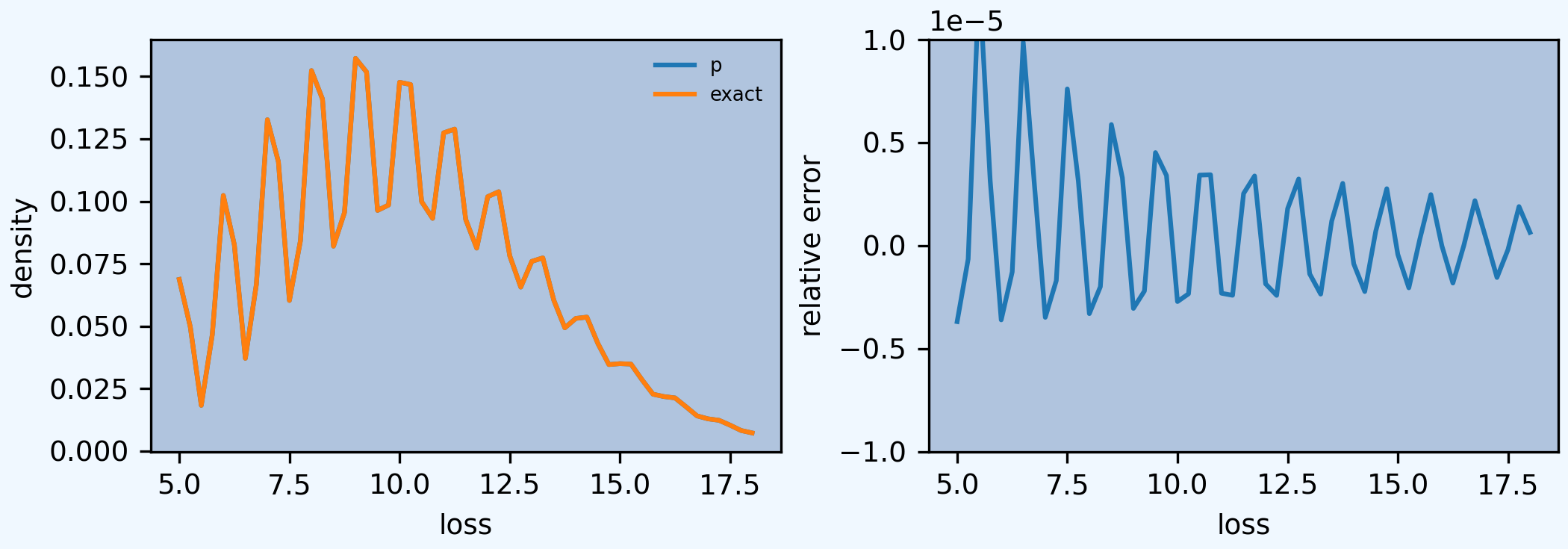
The following graphs show that the FFT approximation is excellent, across a wide range, just as its good moment-matching performance suggests it would be.
In [48]: bit = a.density_df.loc[5:a.q(0.99):256, ['p']]

In [49]: bit['exact'] = [tweedie_density(i, 10, 1.01, 1) for i in bit.index]

In [50]: bit['p'] /= a.bs

In [51]: fig, axs = plt.subplots(1, 2, figsize=(2 * 3.5, 2.45), constrained_layout=True, squeeze=True)

In [52]: ax0, ax1 = axs.flat

In [53]: bit.plot(ax=ax0);

In [54]: ax0.set(ylabel='density');

In [55]: bit['err'] = bit.p / bit.exact - 1

In [56]: bit.err.plot(ax=ax1);

In [57]: ax1.set(ylabel='relative error', ylim=[-1e-5, 1e-5]);