2.4.6. Mixed Severity Distributions
Prerequisites: Examples use build and qd, and basic Aggregate output.
The variables in the severity clause (scale, location, distribution ID, shape parameters, mean and CV) can be vectors to create a mixed severity distribution. All elements are broadcast against one-another.
Example:
sev lognorm 1000 cv [0.75 1.0 1.25 1.5 2] wts [0.4, 0.2, 0.1, 0.1, 0.1]
expresses a mixture of five lognormals, each with a mean of 1000 and CVs equal to 0.75, 1.0, 1.25, 1.5, and 2, and with weights 0.4, 0.2, 0.1, 0.1, 0.1. Equal weights are expressed
as wts=5, or the relevant number of components (note equals sign). A missing weights clause is
interpreted as giving each severity weight 1 which results in five times the
total loss. Commas in the lists are optional.
Warning
Weights are applied to exposure, and their meaning depends on how exposure is entered.
If exposure is given by claim count, then the weights apply to claim count. This gives the usual mixture of severity curves. However, if exposure is entered as loss or premium times a loss ratio, then the weights give the proportion of expected loss, not the claim count. Make sure the weights are appropriate to the way exposure is expressed. For example, if the mixture is used to split small and large claims, then an 80/20 split small/large claim counts may well correspond to a 20/80 split of expected losses (Pareto rule of thumb).
Example.
This example illustrates the different behaviors of wts.
The weights adjust claim counts for each mixture component when exposures are given by claims.
In [1]: from aggregate import build, qd

In [2]: a01 = build('agg DecL:01 '
   ...:             '100 claims '
   ...:             '5000 xs 0 '
   ...:             'sev lognorm [10 20 50 75 100] '
   ...:             'cv [0.75 1.0 1.25 1.5 2] '
   ...:             'wts [0.4, 0.25, 0.15, 0.1, 0.1] '
   ...:             'poisson'
   ...:             , bs=1/2, approximation='exact')
   ...:

In [3]: qd(a01)

       E[X] Est E[X]   Err E[X]   CV(X) Est CV(X)  Skew(X) Est Skew(X)
X
Freq    100                         0.1                0.1
Sev  33.978   33.978 2.5414e-09  2.3807    2.3807   15.161      15.161
Agg  3397.8   3397.8 2.5414e-09 0.25822   0.25822   1.2927      1.2927
log2 = 16, bandwidth = 1/2, validation: not unreasonable.
Mixed severity with Poisson frequency is the same as the sum of five independent components. The report_df shows the mixture details.
In [4]: qd(a01.report_df.iloc[:, :-3])

view              0        1        2        3        4 independent
statistic
name        DecL:01  DecL:01  DecL:01  DecL:01  DecL:01     DecL:01
limit          5000     5000     5000     5000     5000        5000
attachment        0        0        0        0        0           0
el              400      500      750   749.93   997.86      3397.8
freq_m           40       25       15       10       10         100
freq_cv     0.15811      0.2   0.2582  0.31623  0.31623         0.1
freq_skew   0.15811      0.2   0.2582  0.31623  0.31623         0.1
sev_m            10       20       50   74.993   99.786      33.978
sev_cv         0.75        1   1.2498   1.4942   1.9175      2.3807
sev_skew     2.6719        4   5.6619   7.1636   8.3826      15.161
agg_m           400      500      750   749.93   997.86      3397.8
agg_cv      0.19764  0.28284  0.41329  0.56857  0.68386     0.25822
agg_skew    0.30882  0.56568    1.054   1.7191    2.224      1.2927
This aggregate can also be built as a Portfolio.
In [5]: a02 = build(
   ...:     'port DecL:02 '
   ...:         'agg Unit1 40 loss 5000 xs 0 sev lognorm 10 cv 0.75 poisson '
   ...:         'agg Unit2 25 loss 5000 xs 0 sev lognorm 20 cv 1.00 poisson '
   ...:         'agg Unit3 15 loss 5000 xs 0 sev lognorm 50 cv 1.25 poisson '
   ...:         'agg Unit4 10 loss 5000 xs 0 sev lognorm 75 cv 1.50 poisson '
   ...:         'agg Unit5 10 loss 5000 xs 0 sev lognorm 100 cv 2.00 poisson '
   ...:     , bs=1/2, approximation='exact')
   ...:

In [6]: qd(a02)

              E[X] Est E[X]    Err E[X]   CV(X) Est CV(X)  Skew(X) Est Skew(X)
unit  X
Unit1 Freq       4                          0.5                0.5
      Sev       10       10  8.9604e-09    0.75   0.75014   2.6719      2.6704
      Agg       40       40  8.9606e-09   0.625   0.62504  0.97656     0.97653
Unit2 Freq    1.25                      0.89443            0.89443
      Sev       20       20 -9.7705e-09       1         1        4      3.9997
      Agg       25       25 -9.7705e-09  1.2649    1.2649   2.5298      2.5298
Unit3 Freq     0.3                       1.8257             1.8257
      Sev       50       50 -1.0074e-09  1.2498    1.2498   5.6619      5.6618
      Agg       15       15 -1.0074e-09  2.9224    2.9224   7.4526      7.4526
Unit4 Freq 0.13335                       2.7385             2.7385
      Sev   74.993   74.993 -4.0382e-10  1.4942    1.4942   7.1636      7.1635
      Agg       10       10 -4.0383e-10  4.9237    4.9237   14.887      14.887
Unit5 Freq 0.10021                       3.1589             3.1589
      Sev   99.786   99.786  1.1018e-08  1.9175    1.9175   8.3826      8.3826
      Agg       10       10  1.1019e-08  6.8313    6.8313   22.216      22.216
total Freq  5.7836                      0.41582            0.41582
      Sev    17.29    17.29  2.0519e-09  2.2699                 26
      Agg      100      100   2.031e-09  1.0314    1.0314   8.7339      8.7338
log2 = 16, bandwidth = 1/2, validation: not unreasonable.
Actual frequency equals total frequency times weight. Setting wts=5 results in equal weights, here 0.2.
In [7]: a03 = build('agg DecL:03 '
   ...:             '100 claims '
   ...:             '5000 xs 0 '
   ...:             'sev lognorm [10 20 50 75 100] '
   ...:             'cv [0.75 1.0 1.25 1.5 2] '
   ...:             ' wts=5 '
   ...:             'poisson'
   ...:             , bs=1/2, approximation='exact')
   ...:

In [8]: qd(a03)

       E[X] Est E[X]   Err E[X]   CV(X) Est CV(X)  Skew(X) Est Skew(X)
X
Freq    100                         0.1                0.1
Sev  50.956   50.956 3.5836e-09  2.1341    2.1341   11.891      11.891
Agg  5095.6   5095.6 3.5835e-09 0.23568   0.23568  0.99494     0.99494
log2 = 16, bandwidth = 1/2, validation: not unreasonable.
Missing weights are set to 1, resulting in five times loss. This behavior is generally not what you want!
In [9]: a04 = build('agg DecL:04 '
   ...:             '100 claims '
   ...:             '5000 xs 0 '
   ...:             'sev lognorm [10 20 50 75 100] '
   ...:             'cv [0.75 1.0 1.25 1.5 2] '
   ...:             'poisson'
   ...:             , bs=1, approximation='exact')
   ...:

In [10]: qd(a04)

       E[X] Est E[X]    Err E[X]    CV(X) Est CV(X)  Skew(X) Est Skew(X)
X
Freq    500                      0.044721           0.044721
Sev  50.956   50.956 -2.2323e-08   2.1341    2.1341   11.891      11.891
Agg   25478    25478 -2.2323e-08   0.1054    0.1054  0.44495     0.44495
log2 = 16, bandwidth = 1, validation: not unreasonable.
If exposures are determined via losses (directly or using premium and loss ratio or exposure and rate), then the weights apply to expected loss. The resulting mixture is quite different.
In [11]: a01e = build('agg DecL:01e '
   ....:              f'{a01.agg_m} loss '
   ....:              '5000 xs 0 '
   ....:              'sev lognorm [10 20 50 60 70] '
   ....:              'cv [0.75 1.0 1.25 1.5 2] '
   ....:              'wts [0.4, 0.25, 0.15, 0.1, 0.1] '
   ....:              'poisson'
   ....:              , bs=1/2, approximation='exact')
   ....:

In [12]: qd(a01e)

       E[X] Est E[X]   Err E[X]    CV(X) Est CV(X)  Skew(X) Est Skew(X)
X
Freq  115.2                     0.093168           0.093168
Sev  29.493   29.493 1.1694e-08   2.1101    2.1101   14.661      14.661
Agg  3397.8   3397.8 1.1694e-08  0.21755   0.21755    1.113       1.113
log2 = 16, bandwidth = 1/2, validation: not unreasonable.

In [13]: qd(a01e.report_df.iloc[:, :-3])

view               0         1         2         3         4 independent
statistic
name        DecL:01e  DecL:01e  DecL:01e  DecL:01e  DecL:01e    DecL:01e
limit           5000      5000      5000      5000      5000        5000
attachment         0         0         0         0         0           0
el            460.82    576.02    864.03     691.2    805.71      3397.8
freq_m        46.082    28.801    17.281     11.52     11.52       115.2
freq_cv      0.14731   0.18634   0.24056   0.29462   0.29462    0.093168
freq_skew    0.14731   0.18634   0.24056   0.29462   0.29462    0.093168
sev_m             10        20        50    59.997    69.938      29.493
sev_cv          0.75         1    1.2498    1.4968    1.9523      2.1101
sev_skew      2.6719         4    5.6619    7.3823    9.6027      14.661
agg_m         460.82    576.02    864.03     691.2    805.71      3397.8
agg_cv       0.18414   0.26352   0.38505   0.53034   0.64624     0.21755
agg_skew     0.28772   0.52703   0.98195    1.6404    2.3418       1.113
2.4.6.1. Mixed Exponential Distributions
The mixed exponential distribution (MED) is used by major US rating
bureaus to model severity and compute increased limits factors (ILFs).
This example explains how to create a MED in aggregate. The
distribution is initially created as an Aggregate object with a degenerate
frequency identically equal to 1 claim to focus on the severity.
We then explain how frequency mixing interacts with a mixed severity.
The next table of exponential means and weights appears on slide 24 of Li Zhu, Introduction to Increased Limits Factors, 2011 RPM Basic Ratemaking Workshop,, titled a “Sample of Actual Fitted Distribution”. At the time, it was a reasonable curve for US commercial auto. We will use these means and weights.
Here the DecL to create this mixture.
In [14]: med = build('agg Decl:MED '
   ....:             '1 claim '
   ....:             'sev [2.764e3 24.548e3 275.654e3 1.917469e6 10e6] * '
   ....:             'expon 1 '
   ....:             'wts [0.824796 0.159065 0.014444 0.001624, 0.000071] '
   ....:             'fixed')
   ....:

In [15]: qd(med)

      E[X] Est E[X]  Err E[X]  CV(X) Est CV(X) Skew(X) Est Skew(X)
X
Freq     1                         0
Sev  13990    13798 -0.013708 12.034    12.203  103.79      103.76
Agg  13990    13798 -0.013708 12.034    12.203  103.79      103.76
log2 = 16, bandwidth = 4000, validation: fails sev mean, agg mean.
Note
Currently, it is necessary to enter a dummy shape parameter 1 for the exponential, even though it does not take a shape. This is a known bug in the parser.
The exponential distribution is surprisingly thick-tailed. It can be
regarded as the dividing line between thin and thick tailed distributions.
In order to achieve good accuracy, the modeling increases the number of
buckets to \(2^{18}\) (i.e., log2=18) and uses a bucket size bs=500.
The dataframe report_df is a more detailed version of the audit dataframe
that includes information from statistics_df about each severity component.
(The reported claim counts are equal to the weights and cannot be interpreted
as fixed frequencies. They can be regarded as frequencies for a Poisson or
mixed Poisson.)
In [16]: med.update(log2=18, bs=500)

In [17]: qd(med)

      E[X] Est E[X]    Err E[X]  CV(X) Est CV(X) Skew(X) Est Skew(X)
X
Freq     1                           0
Sev  13990    13987 -0.00022819 12.034    12.037  103.79      103.72
Agg  13990    13987 -0.00022819 12.034    12.037  103.79      103.72
log2 = 18, bandwidth = 500, validation: fails sev mean, agg mean.
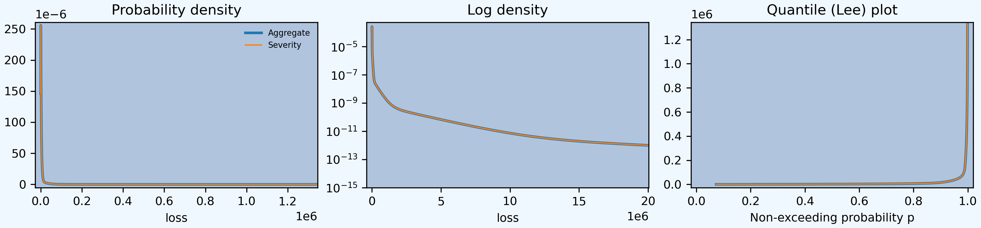
The middle diagnostic plot, the log density, shows the mixture components.
In [18]: med.plot()
The density_df dataframe includes a column lev. From this we can pull
out ILFs. Zhu reports the ILF at 1M equals 1.52.
In [19]: qd(med.density_df.loc[1000000, 'lev'] / med.density_df.loc[100000, 'lev'])
1.5204
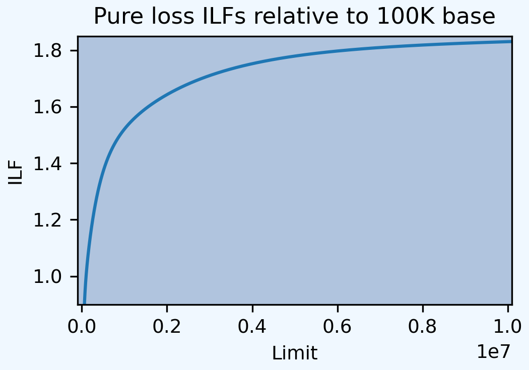
Here is a graph of the ILFs by limit.
In [20]: base = med.density_df.loc[100000, 'lev']

In [21]: ax = (med.density_df.lev / base).plot(xlim=[-100000,10.1e6], ylim=[0.9, 1.85],
   ....:                                       figsize=(3.5, 2.45))
   ....:

In [22]: ax.set(xlabel='Limit', ylabel='ILF', title='Pure loss ILFs relative to 100K base');
2.4.6.2. Saving to the Knowledge
We can save the MED severity in the knowledge and then refer to it by name.
In [23]: build('sev COMMAUTO [2.764e3 24.548e3 275.654e3 1.917469e6 10e6] * '
   ....:       ' expon 1 wts [0.824796 0.159065 0.014444 0.001624, 0.000071]');
   ....:

In [24]: a05 = build('agg DecL:05 [20 8 4 2] claims [1e6, 2e6 5e6 10e6] xs 0 '
   ....:                   'sev sev.COMMAUTO fixed',
   ....:                   log2=18, bs=500)
   ....:

In [25]: qd(a05)

           E[X]   Est E[X]    Err E[X]  CV(X) Est CV(X) Skew(X) Est Skew(X)
X
Freq         34                             0
Sev       11973      11970 -0.00026506  6.328    6.3298  31.665      31.665
Agg  4.0708e+05 4.0697e+05 -0.00026506 1.0852    1.0855  5.4306      5.4305
log2 = 18, bandwidth = 500, validation: fails sev mean, agg mean.
2.4.6.3. Different Distributions
The kind of distribution can vary across mixtures. In the following, exposure varies for each curve, rather than using weights, see Vectorization: Limit Profiles and Mixed Severity.
In [26]: a06 = build('agg DecL:06 [100 200] claims '
   ....:             '5000 xs 0 '
   ....:             'sev [gamma lognorm] [100 150] cv [1 0.5] '
   ....:             'mixed gamma 0.5',
   ....:             log2=16, bs=2.5)
   ....:

In [27]: qd(a06.report_df.iloc[:, :-2])

view              0        1 independent    mixed
statistic
name        DecL:06  DecL:06     DecL:06  DecL:06
limit          5000     5000        5000     5000
attachment        0        0           0        0
el            10000    30000       40000    40000
freq_m          100      200         300      300
freq_cv      0.5099  0.50498     0.37712  0.50332
freq_skew    1.0002        1     0.80295        1
sev_m           100      150      133.33   133.33
sev_cv            1      0.5     0.65551  0.65551
sev_skew          2    1.625      1.4508   1.4508
agg_m         10000    30000       40000    40000
agg_cv      0.51962  0.50621     0.40127  0.50474
agg_skew     1.0022   1.0002     0.88112   1.0001

In [28]: a06.plot()
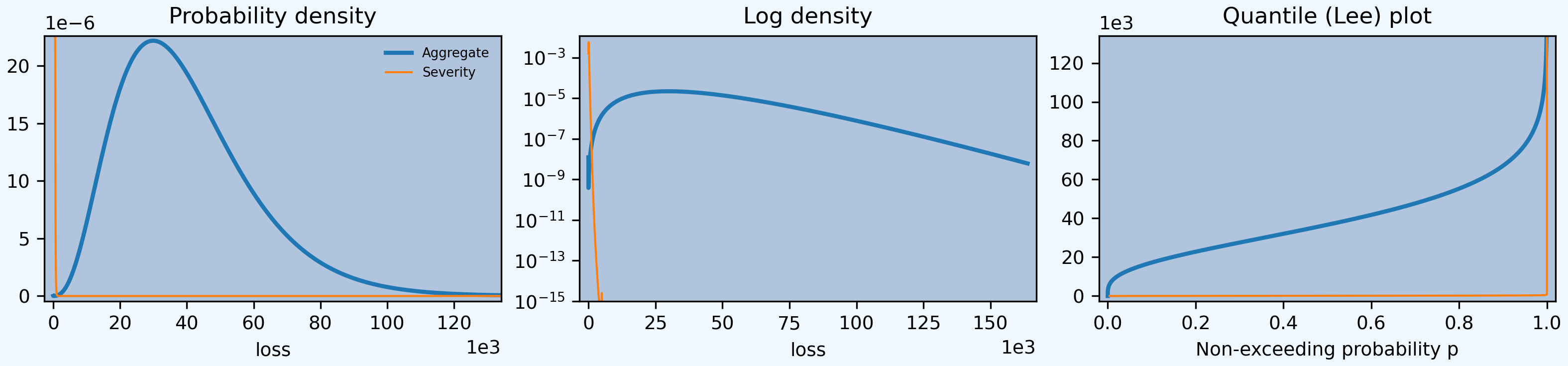
Using a Delaporte (shifted) gamma mixing often produces more realistic output than a gamma, avoiding very good years.
In [29]: a07 = build('agg DecL:07 [100 200] claims '
   ....:              '5000 xs 0 '
   ....:              'sev [gamma lognorm] [100 150] cv [1 0.5] '
   ....:              'mixed delaporte 0.5 0.6',
   ....:             log2=18, bs=2.5)
   ....:

In [30]: qd(a07.report_df.iloc[:, :-2])

view              0        1 independent    mixed
statistic
name        DecL:07  DecL:07     DecL:07  DecL:07
limit          5000     5000        5000     5000
attachment        0        0           0        0
el            10000    30000       40000    40000
freq_m          100      200         300      300
freq_cv      0.5099  0.50498     0.37712  0.50332
freq_skew    2.4145   2.4561      1.9682   2.4705
sev_m           100      150      133.33   133.33
sev_cv            1      0.5     0.65551  0.65551
sev_skew          2    1.625      1.4508   1.4508
agg_m         10000    30000       40000    40000
agg_cv      0.51962  0.50621     0.40127  0.50474
agg_skew     2.3386   2.4456      2.1507   2.4582

In [31]: a07.plot()

2.4.6.4. Severity Mixtures and Mixed Frequency
All severity components in an aggregate share the same frequency mixing value, inducing correlation between the parts. An Aon study, Aon Benfield [2015], shows that commercial auto has parameter uncertainty CV around 25%. Building with
In [32]: a08 = build('agg DecL:08 '
   ....:             '500 claims '
   ....:             '500000 xs 0 sev sev.COMMAUTO '
   ....:             'poisson'
   ....:             , approximation='exact')
   ....:

In [33]: a09 = build('agg DecL:09 '
   ....:             '500 claims '
   ....:             '500000 xs 0 sev sev.COMMAUTO '
   ....:             'mixed gamma 0.25'
   ....:             , approximation='exact')
   ....:

In [34]: qd(a08)

           E[X]   Est E[X]    Err E[X]    CV(X) Est CV(X)  Skew(X) Est Skew(X)
X
Freq        500                        0.044721           0.044721
Sev       10266      10266 -4.9496e-05   3.9519    3.9522   9.4914      9.4913
Agg  5.1332e+06 5.1329e+06 -4.9496e-05  0.18231   0.18232  0.41833     0.41833
log2 = 16, bandwidth = 200, validation: not unreasonable.

In [35]: qd(a09)

           E[X]   Est E[X]   Err E[X]   CV(X) Est CV(X)  Skew(X) Est Skew(X)
X
Freq        500                       0.25397            0.50006
Sev       10266      10264 -0.0001979  3.9519    3.9528   9.4914       9.491
Agg  5.1332e+06 5.1321e+06 -0.0001979 0.30941   0.30943  0.55969      0.5597
log2 = 16, bandwidth = 400, validation: fails sev mean, agg mean.
The effect of shared mixing is shown in report_df. In order to focus on the mixing and ease the computational
burden, apply a 500,000 policy limit to model a self-insured retention.
Assume a claim count of 500 claims; for smaller portfolios the impact of mixing is less pronounced because idiosyncratic process risk dominates.
The independent column in report_df shows statitics assuming the mixture components are independent; mixed includes the effect of shared mixing variables.
The next block shows results with a Poisson frequency, where there is no mixing. The independent and mixed columns are identical.
In [36]: qd(a08.report_df.drop(['name']).iloc[:, :-2])

view                0          1          2          3          4 independent      mixed
statistic
limit           5e+05      5e+05      5e+05      5e+05      5e+05       5e+05      5e+05
attachment          0          0          0          0          0           0          0
el         1.1399e+06 1.9524e+06 1.6662e+06 3.5738e+05      17314  5.1332e+06 5.1332e+06
freq_m          412.4     79.532      7.222      0.812     0.0355         500        500
freq_cv      0.049243    0.11213    0.37211     1.1097     5.3074    0.044721   0.044721
freq_skew    0.049243    0.11213    0.37211     1.1097     5.3074    0.044721   0.044721
sev_m            2764      24548 2.3072e+05 4.4013e+05 4.8771e+05       10266      10266
sev_cv              1          1    0.73847    0.29449    0.12909      3.9519     3.9519
sev_skew            2          2    0.39392     -2.071    -5.6054      9.4914     9.4914
agg_m      1.1399e+06 1.9524e+06 1.6662e+06 3.5738e+05      17314  5.1332e+06 5.1332e+06
agg_cv        0.06964    0.15858    0.46257     1.1569     5.3515     0.18231    0.18231
agg_skew      0.10446    0.23787    0.54133     1.1826     5.3739     0.41833    0.41833
This block shows mixed gamma (negative binomial) frequency. There are two differences: the individual components have higher CVs (they asymptotically approach 25% for a large portfolio), and the mixed column includes correlation between units (aggregate CV is greater than independent). Glenn Meyers had the idea of using shared mixing variables to ensure aggregate portfolio dynamics are not influenced by how the portfolio is split into units.
In [37]: qd(a09.report_df.drop(['name']).iloc[:, :-2])

view                0          1          2          3          4 independent      mixed
statistic
limit           5e+05      5e+05      5e+05      5e+05      5e+05       5e+05      5e+05
attachment          0          0          0          0          0           0          0
el         1.1399e+06 1.9524e+06 1.6662e+06 3.5738e+05      17314  5.1332e+06 5.1332e+06
freq_m          412.4     79.532      7.222      0.812     0.0355         500        500
freq_cv        0.2548      0.274    0.44829     1.1376     5.3133     0.21474    0.25397
freq_skew     0.50009     0.5021    0.58771     1.1925     5.3251       0.473    0.50006
sev_m            2764      24548 2.3072e+05 4.4013e+05 4.8771e+05       10266      10266
sev_cv              1          1    0.73847    0.29449    0.12909      3.9519     3.9519
sev_skew            2          2    0.39392     -2.071    -5.6054      9.4914     9.4914
agg_m      1.1399e+06 1.9524e+06 1.6662e+06 3.5738e+05      17314  5.1332e+06 5.1332e+06
agg_cv        0.25952    0.29605    0.52581     1.1836     5.3573     0.22858    0.30941
agg_skew      0.50102    0.51935     0.6983     1.2604     5.3913     0.42255    0.55969